 Marco Russo & Alberto Ferrari
Do you know the (not so) secret ingredient of the perfect Power BI model? The one detail that seasoned developers never forget to add to their projects, while newbies underestimate it quite often? The star schema.
Business Intelligence changed over the years. Nearly everything has been updated with new technologies and new software. The one thing that never changed is how to model your data to obtain a fast, reliable, and easy-to-use solution. In the age of cloud computing, columnar databases, in-memory data models, and fancy user interfaces, a star schema is still the best option. For one single reason: it works better than anything else.
We already shown in a previous article (Power BI – Star schema or single table – SQLBI) how the star schema proves to be the best option when compared with a single table model. Single-table models are the evil: do not be tempted by them, choose a star schema.
In this article, I want to show you an example in the opposite direction. A single table model denormalizes everything in one table, and we already learned that it is bad. But what if we keep a more normalized structure, as it often happens in header/detail models (like orders and order lines)? Is a header/detail model better than a star schema? The quick answer is: “No. Nope. No way. Not at all. Are you kidding me? No.”. Nonetheless, this might be just our personal opinion. The goal of the article is to provide you with some numbers and considerations to prove the previous statement.
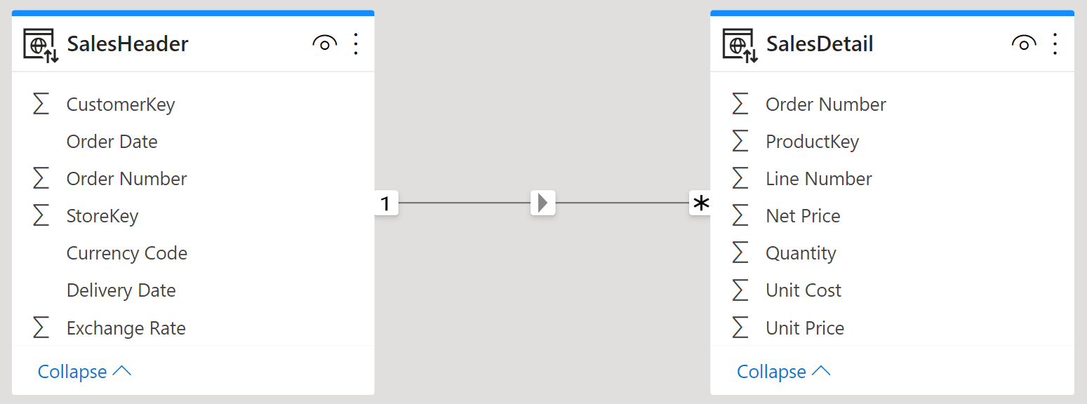
Let us start by understanding why we have header/detail models. Header/detail structures appear very often in source models. You might have invoices, and invoice details. An invoice has a date, a customer, a store and many more information that make sense at the invoice level. The detail contains the product, the net price, the quantity, and other pieces of information related to the individual invoice line. As such, it seems reasonable to create two tables: SalesHeader and SalesDetail. Each table contains the relevant columns for the entity it is storing, and a relationship exists between the two tables:
Despite this model being the most natural one, it is also the wrong one for analytical purposes. Let me elaborate on this.
First, from a purely modeling point of view, both SalesHeader and SalesDetail are fact tables. If you look at the model from farther away, you see that both tables are linked to dimensions, as it needs to be. This simple fact makes both tables fact tables.
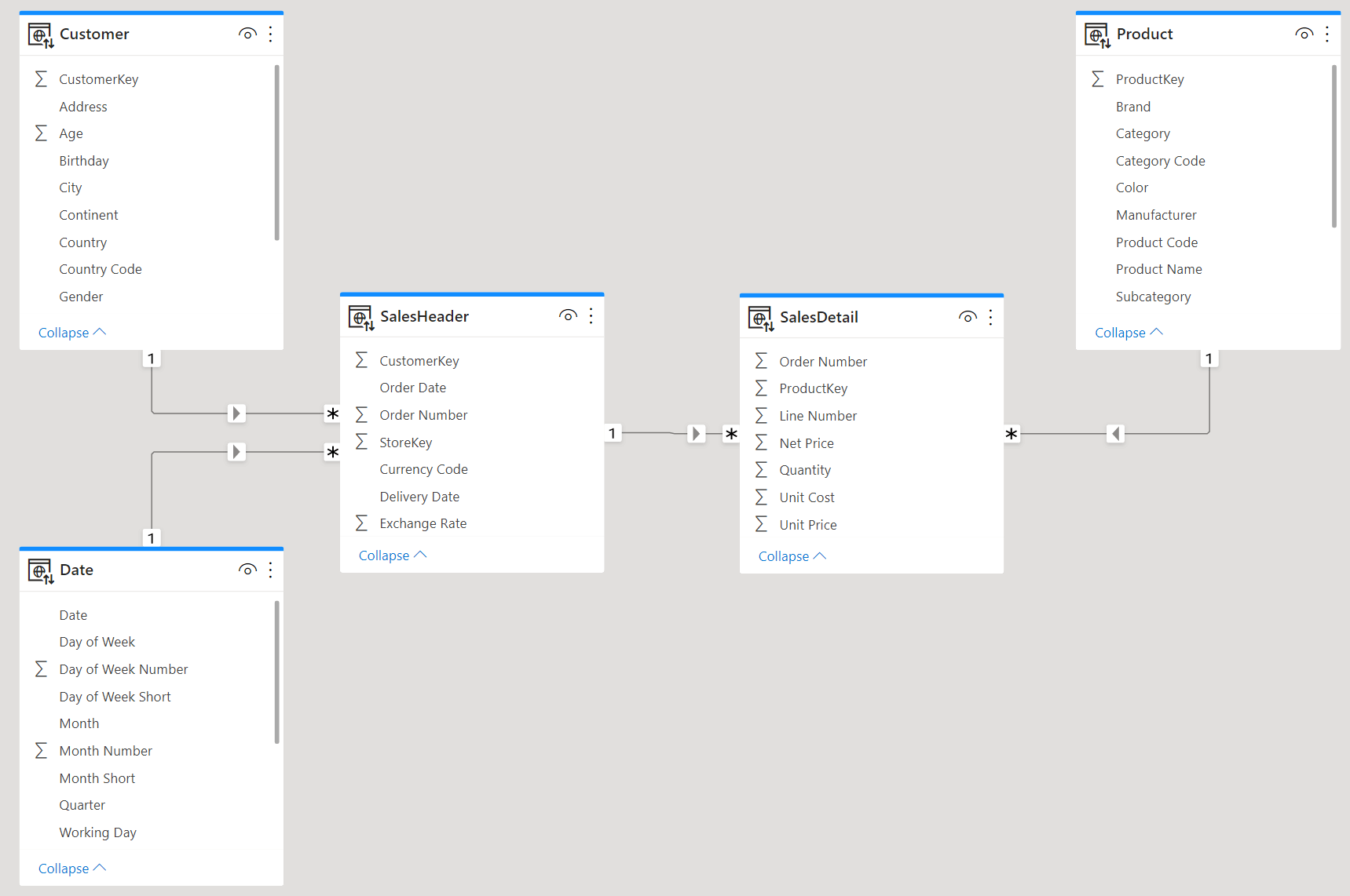
Therefore, the relationship between SalesHeader and SalesDetail is a relationship between two fact tables. This is forbidden by the star schema rules. Therefore, this model is not a star schema.
The correct model, for such a structure, requires moving all the information stored in SalesHeader into SalesDetail. SalesDetail becomes, at this point, a single fact table linked to all the dimensions. As such, we can call it just Sales, as we are used to:
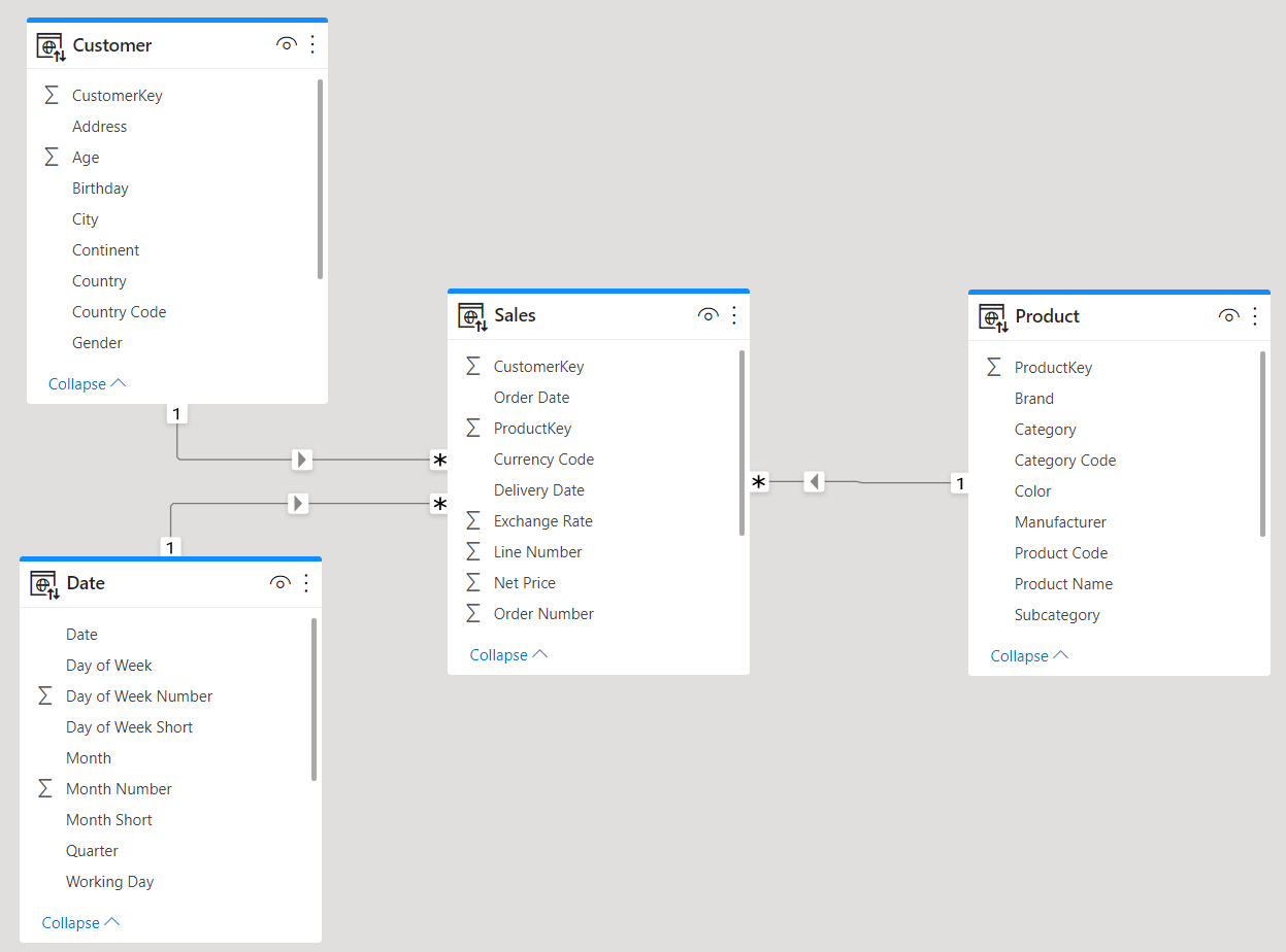
This last model is a pure star schema. Nonetheless, if the source model you are loading from is designed as a header/detail model, then building this star schema requires some extra effort.
This brings us to the next question: is it worth writing the code required to transform a header/detail source model into a pure star schema? This time, the answer is not “it depends”. It is a clear and strong “yes”. It is definitely worth. There are modeling considerations that we cover in the Introduction to Data Modeling. There are DAX considerations, again covered in the training: the DAX code over the star schema is simpler, better, faster. There are also performance considerations strictly related to how the model is shaped; we cover the performance aspect in this article.
Let us state from the beginning of the analysis where the problem is: the size of the relationship between SalesHeader and SalesDetail. This relationship is based on the Order Number column, that is likely to show a large number of distinct values. The speed of a query involving a relationship strongly depends on the size of the relationship. The larger the relationship, the slower the query is.
We created a model to test the performance. The model contains both the single Sales fact table, and the pair of SalesHeader and SalesDetail tables. In order to appreciate the impact of the relationship, we used a model with around 1.4 billion rows in Sales. Let us start analyzing the size of the header/detail model by using VertiPaq Analyzer:
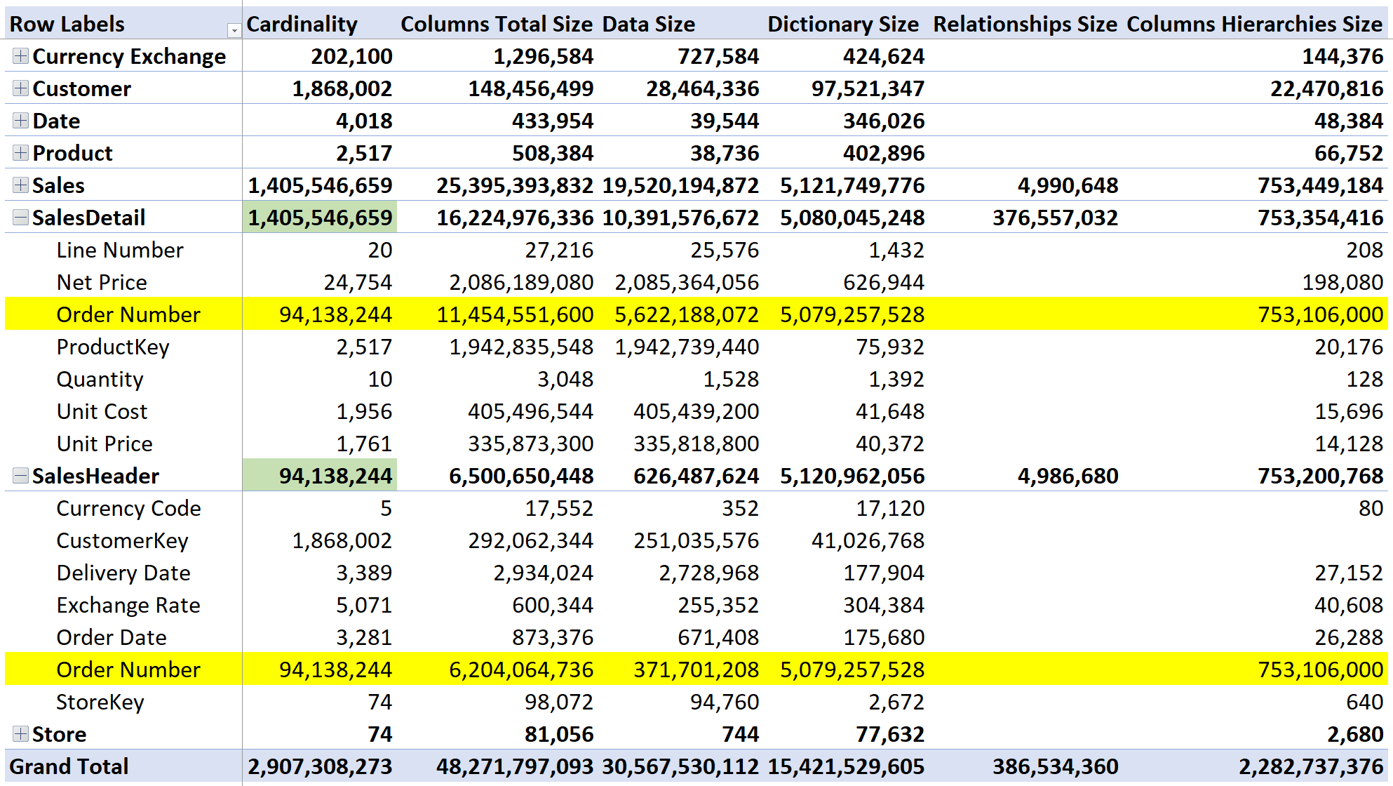
There are 1.4B rows in SalesDetail, with 94M orders. The relevant thing here is the cardinality of Order Number, which is 94,138,244 rows. There are two columns containing the Order Number: one in SalesDetail and one in SalesHeader. The total size required for the column is 11,454,551,600 plus 6,204,064,736 bytes, resulting in 17,658,616,336 bytes used (17 GB). The dictionary size is quite relevant because the order number is stored as a string. Nonetheless, as you see, size matters in this model. Whenever the engine needs to traverse the relationship, it has to deal with large data structures and this simple fact is affecting performance.
In their entirety, the two tables account for 22 GB, 17 of which are used for the relationship. Let us now look at the Sales table, that contains the same information in a single table:
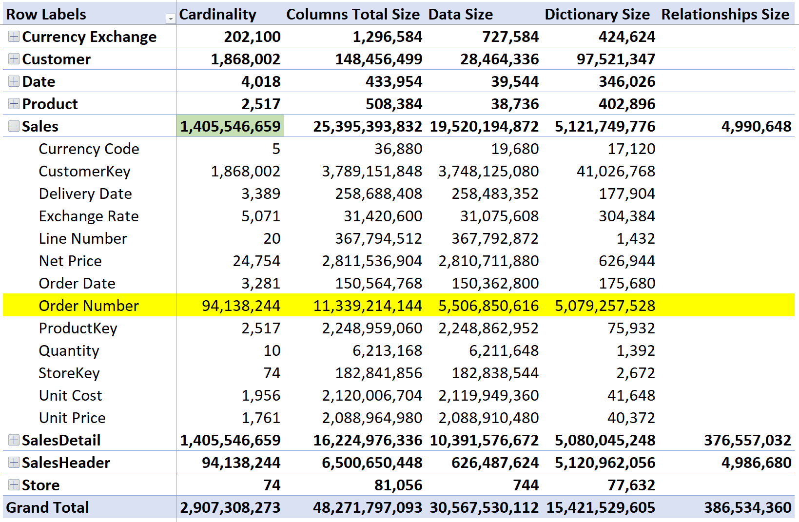
As you see, the size of the column is comparable to the same column in SalesDetail. In this structure, nonetheless, Order Number exists only once. Despite having a single column, the overall size is larger. Indeed, the Sales table uses 25 GB of RAM, three more than the 22 GB used by the pair of tables.
This first result is expected. Normalized structures result in being smaller than denormalized ones. Sales contains all the columns in SalesDetail, but they are repeated multiple times. Indeed, SalesHeader is two orders of magnitude smaller than both Sales and SalesDetail.
Your mileage might vary by a lot regarding the size of the model. In this demo file, we are observing around 15% more space being used in the star schema. It would not be surprising to see a large variation on this percentage depending on the specifics of your model, both in term of number of columns and data distribution. Nonetheless, the analysis is far from being complete. We evaluated size; we need to test performance. Besides, the most relevant detail of this analysis is not the comparison of the two models but, rather, the size of the Order Number column. It is huge in both scenarios but in Sales it is used only to count the orders, when needed; in the header/details scenario it is used for any query, because the Order Number column is the means to move a filter from Customer to SalesDetail, through SalesHeader. As you see, the usage of the column in the two scenario is very different. Hence, performance is going to be very different too.
Testing performance is not complex in this scenario. It is enough to author a query that groups by attributes of the customer and computes values at the higher grain: SalesDetail or Sales. When the query is executed over Sales, you pay the price of the relationship between Customer and Sales. When the query is executed over SalesDetail, you have the additional price of the relationship between SalesHeader and SalesDetail. All other parts of the query are totally identical. Therefore, if the query over SalesDetail results in being slower, we are measuring exactly the additional price of the relationship.
Here is the full query. We executed first the calculation with Amt S, that scans Sales, and later the calculation with Amt H, that involves the header/detail structure:
EVALUATE
SUMMARIZECOLUMNS (
    'Customer'[Country],
    "Amt S",
        SUMX (
            Sales,
            Sales[Quantity] * Sales[Net Price]
        ),
    "Amt H",
        SUMX (
            SalesDetail,
            SalesDetail[Quantity] * SalesDetail[Net Price]
        )
)
This is the result of Amt S:
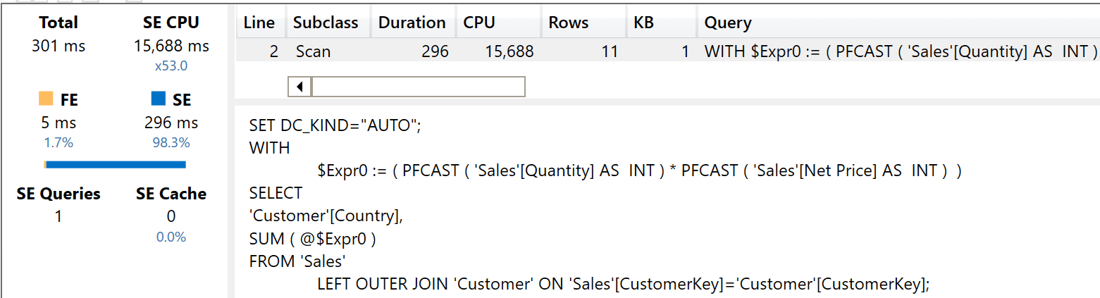
The query uses 15,688 milliseconds of CPU with the storage engine. The total execution time obviously depends on the number of cores of the server running the model. The execution of Amt H proves to be very different:
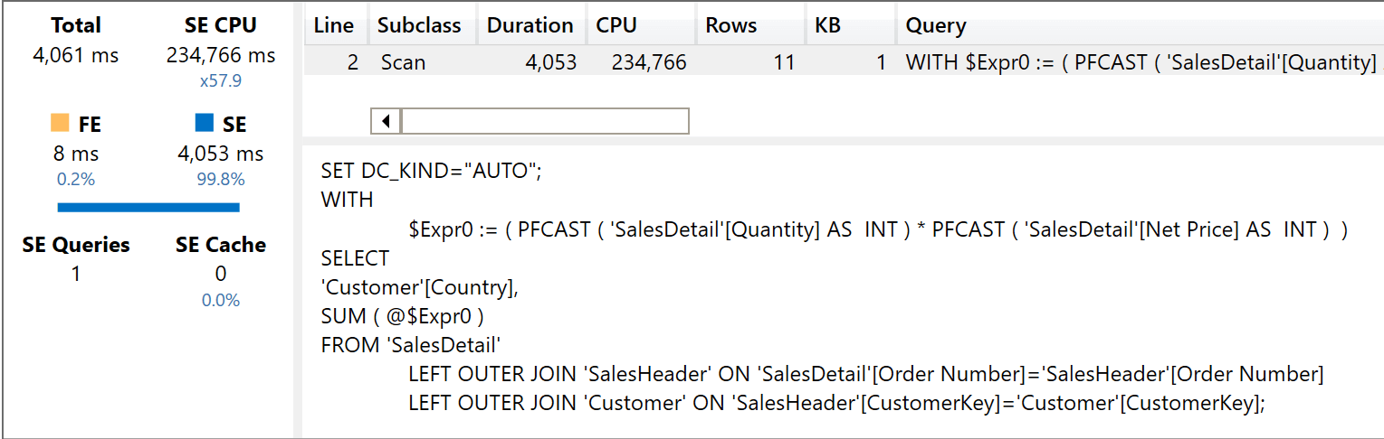
The Storage Engine CPU time skyrocketed to 234,766 milliseconds. You can also clearly see, in the xmSQL query that there are now two joins: one with Customer, as it happened with the previous query, and one with SalesHeader.
In short, the header/detail model uses 15 times more CPU than the star schema. In this scenario, the ratio is very high because the calculation is rather simple, involving only one multiplication and a sum. If the calculation were more complex, the ratio will likely be smaller. Nonetheless, the high-cardinality relationship is simply ridiculously expensive in terms of performance.
Finally, keep in mind that this price needs to be paid whenever you need to traverse the relationship between SalesHeader and SalesDetail. If you browse both tables slicing by columns in Product, for example, performance is similar. As soon as you filter one year, or slice by customer continent, the relationship between the two fact tables comes into play, resulting in extremely poor performance.
This is not to say that the idea of using an SalesHeader table is completely rubbish. There are scenarios where you actually want to create a SalesHeader table to optimize specific calculations. It is quite expensive in terms of RAM used, but it can produce great results.
For example, if you need to compute the distinct count of buying customers sliced by Country, the two structures provide again very different performance, this time in favor of the header/detail. Indeed, by using the SalesHeader table, you can compute the number of customers. Here is the test query:
EVALUATE
SUMMARIZECOLUMNS(
    'Customer'[Country],
    "Cus S", DISTINCTCOUNT ( Sales[CustomerKey] ),
    "Cus H", DISTINCTCOUNT ( SalesHeader[CustomerKey] )
)
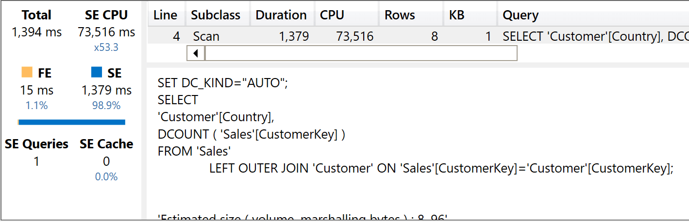
And here are the results, first with the star schema:
And then with the header/detail:
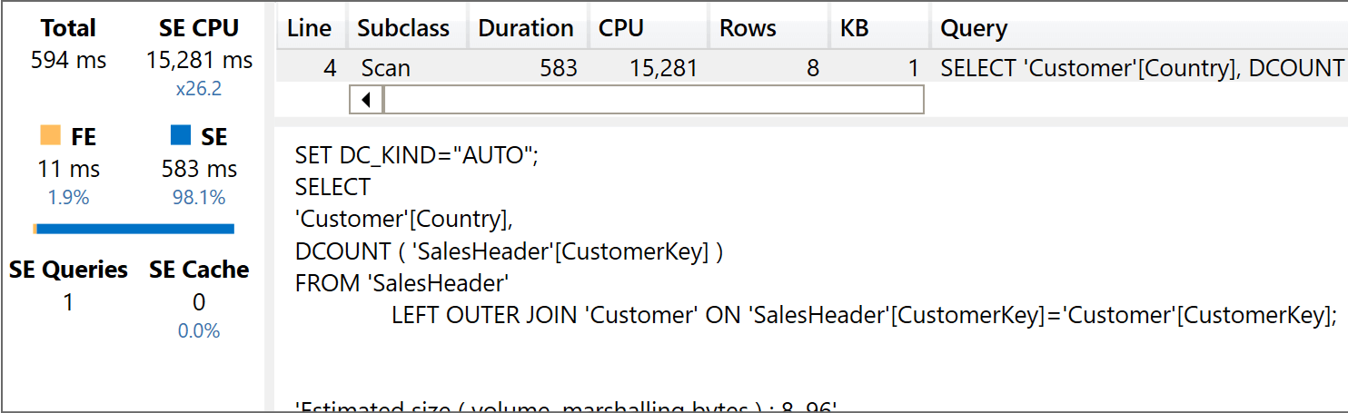
The query using the star schema uses 73,516 milliseconds of SE CPU, whereas the query using the header/detail uses only 15,281 milliseconds of SE CPU. Therefore, the header/detail model is around five times faster. Nonetheless, you are limited by the distinct count over attributes that can be reached through dimensions linked to SalesHeader only. As soon as you want to slice the previous query by Product[Brand], then you need to turn the relationship between SalesHeader and SalesDetail as a bidirectional one, vanishing the benefit entirely. The following query has been executed with the relationship between SalesHeader and SalesDetail set as bidirectional:
EVALUATE
SUMMARIZECOLUMNS (
    Customer[Country],
    'Product'[Brand],
    "Cus S", DISTINCTCOUNT ( Sales[CustomerKey] ),
    "Cus H", DISTINCTCOUNT ( SalesHeader[CustomerKey] )
)
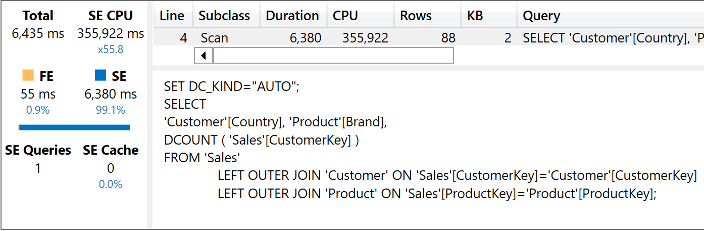
As we did earlier, first the version with the star schema:
And then the code executed against the header/detail model:
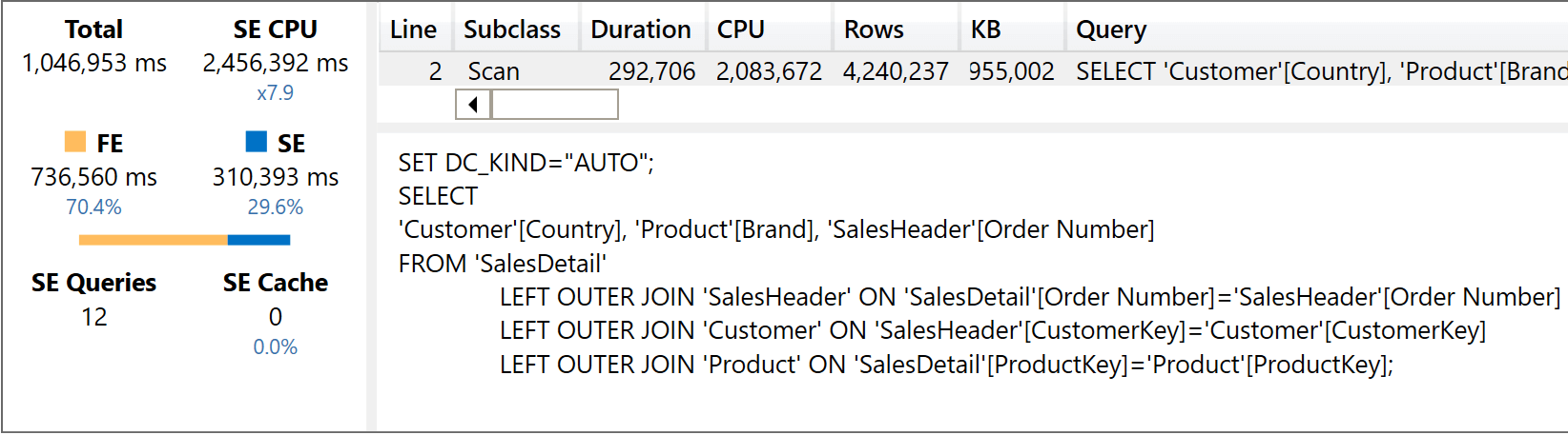
The version with the star schema is consistent with the previous executions, providing the result after having used 355,922 milliseconds of SE CPU. The version that needs to traverse the large, bidirectional relationship is incredibly slow: it used 2,456,392 milliseconds of SE CPU and 1,046,953 milliseconds of FE CPU. We save you the math: it is around 17 minutes, because the formula engine is single-threaded.
Conclusions
We have seen several considerations and measurements taken on both models. The header/detail model is slightly smaller, and, at first sight, it looks tempting. That said, when you measure performance the header/detail model goes from bad to ugly, if compared with the star schema.
Clearly, on smaller models the difference might be less noticeable. Nonetheless: don’t be fooled. Even though performance might seem similar because the size of your data is way smaller than the 1.4B rows we used for testing, still the header/detail model is performing poorly. In other words, you are wasting precious (and expensive) CPU power because of a poor data model.
There are good reasons why old and seasoned data modelers always choose a star schema for their models. This example is just another one. Let us say: quite a powerful one.