PowerPivot, basket analysis and the hidden many to many

Surfing on the web, here, I came into this intriguing question:

How do we ask something like “Show me how many customers have an iPad but don’t have a book?”

We are speaking about a sales analysis where the canonical entities are Customers, Products and Sales. Moreover, because we have been used to speak about cycles since many years ago, due to the nature of AdventureWorks, the question can be posed in AdventureWorks’s language as:

Of all the customers who have bought a mountain bike, how many have never bought at least one mountain tire tube?

The marketing need to answer this question is evident, if my customers have bought a mountain bike, they need to buy tire tubes. If they don’t buy them from me, it means that they are taking them somewhere else, and this is not good.

There are some interesting points in this simple question that turn the scenario into a challenging one:

We want to filter customers based on sales and then perform further analysis on the behavior of these customers
The simple presence of “not” in the question makes it much more complicated because we will need to check the customer that did not buy tires and this is not very intuitive to compute because we need to search for lacking information
The question has been posed for a single product but it is clear that the customer might want to perform the analysis on categories of products too. Moreover he probably want to be able to slice at the single product level.
Finally, we need to find a generic solution which is easy to query with a PivotTable, because users like Excel

The scenario is an interesting one, definitely worth a post. What about the solution, is it interesting too? It is for one simple reason: in order to solve it we will need to search for a many-to-many relationship where we are not used to find one. Moreover, I love all the solutions that force me to think in DAX and, as we are going to see, the scenario is quite simple in DAX while it would be much more complicated using any other tool. Well… beware that “quite simple” does not mean “simple”, the DAX code is a bit intricate but, hopefully, I am going to help you reading it.

A simple side note: this data model has been developed with PowerPivot but, as the new data modeling paradigm has been disclosed just a few days ago with the name “tabular” in the BISM architecture, I will refer to this as a “tabular data model” to distinguish it from the “multidimensional data model”.

In fact, this scenario is very similar to the survey data model described in the “Many-to-Many revolution” by Marco Russo even if the data structure is not so evident at first glance.

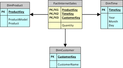
Let us start speaking about the data model. It is a canonical star schema as taken from the AdventureWorks data warehouse:

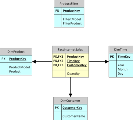
Importing these tables (and their relationships) inside PowerPivot is a good first step but soon we will discover that something is missing. We need to have two instances of the DimProduct table. One is needed to detect the customers who have bought one of the selected product, in our example the mountain bike. The other one will be needed to select the product which we want to check, in our example the tire tubes. Thus, we will need to load the DimProduct twice inside the tabular data model. Because the new instance of DimProduct will be used for filtering, we name it “ProductFilter”.

Thus, the complete data model we are going to work with is the following:

This definitely looks like a strange diagram: the new ProductFilter table has no relationships with the fact table nor with any dimension. In fact, if you think at it carefully, you’ll discover that we have no way to create a relationship between the fact table and the ProductFilter table, because the only available ProductKey in the fact table has already been used for the relationship with DimProduct. Tabular, among its limitations, can use a column for one relationship only. Nevertheless, we don’t care about it: the point is that that relationship is not needed, we will write the DAX code without leveraging its existence.

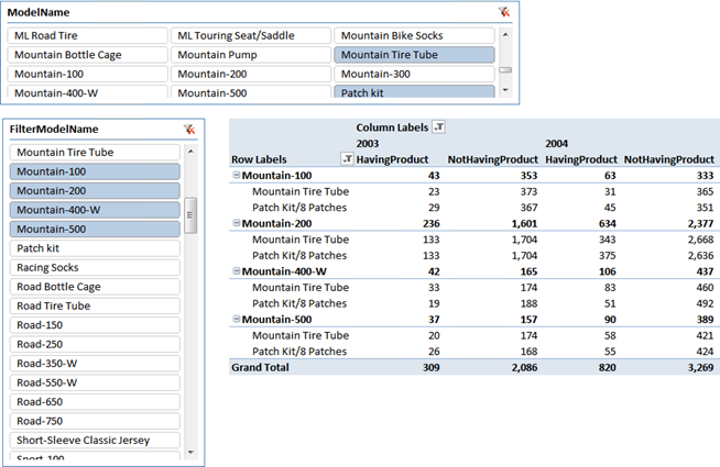
Before to dive into the DAX solution, let us spend some time to describe the desired result. We want to be able to produce a report like this:

In the report, we have selected four model types in the vertical slicer (mountain bikes from 100 to 500) which are the product we require the customer to have bought. Then we have selected two product models in the horizontal slicer (tire tubes and patch kits) which represent the products we want to check whether the customer have bought or not.

On the rows we have put FilterModelName and the ProductName columns. On the columns, as usual, there is the time. The two measures shown are:

HavingProduct: it counts the number of customer who bought a mountain bike and some tire tube or patch kit.
NotHavingProduct: it counts the number of customer who bought a mountain bike but no tire tube nor patch kit.

Due to the nature of the measures, we have decided to make these measures incremental over time. This means that, in 2003, we count all the customers that have bought a mountain bike before the end of 2003 and have bought tire tubes before the same time. In 2004, we perform the same computation, thus including the customers of 2003. It can be changed, but it makes sense to compute the value this way.

Thus, the PivotTable can be read as (first line): 396 (43+353) people have bought a Mountain-100 bicycle before 2003 and, of those, 43 have bought either a mountain tire tube or a patch kit. 353 of them did not buy tires or tubes (at least from us). The same for 2004 and for all other cells.

Ok we spent enough time describing the scenario, it is now time to write some DAX code. Because the final formulas turn out to be quite complicated, we will describe them step by step, trying to figure out the algorithm before giving the final formula.

Let us start with the HavingProduct measure, which is somehow simpler since it does not contain the “not” part.

First of all, we need to compute the set of the customers who have bought a mountain bike before 2003. Let us focus on the worksheet: there is a slicer filtering model names on the ProductFilter table and we want to use this filter to detect the customer who have bought these products. Moreover, the presence of the year on the columns creates a filter on the time table, showing only the sales for 2003. The steps we need to carry on are two:

We need to push the filter from the ProductFilter to the customers, using the fact table as a bridge
We need to extend the filter context on time to show all the time before the end of 2003, since we want “before 2003”

We need to take into account the fact that the scenario is a bit more complicated than what we have spoken so far. In reality, we forgot to speak about the horizontal slicer. Its presence means that the fact table is filtered from the DimProduct too. That filter exists because there is a relationship between DimProducts and the fact table. Moreover, remember that our task is to push the filter on ProductFilter to the DimCustomer, passing through the fact table and there are no relationships between ProductFilter and the fact table. It comes out that the fact table, for our first task, is automatically filtered by the wrong product dimension.

Now, with all these considerations in mind, the algorithm looks like:

For each customer
- For each product
- Check if there are sales
  - Of at least one of the products selected in ProductFilter
  - Anytime before the end of the currently selected year

The key of the solution is to think at the fact table as being a bridge table that implements a many-to-many relationship between customers and products. While sales are not usually intended to implement this relationship, it is clear that this relationship holds. Thus, for each customer, we can filter the fact table showing only the sales of that customer, of the products selected in ProductFilter and of the dates before the end of the current year. If there exists at least one row, this means that that customer has bought one of the ProductFilter products. But, remember that the fact (now bridge) table is already filtered by the wrong product dimension. Thus, we need to remove that filter and replace it with the one we want to use.

Although non very easy, the formula that detects these customers should now be understandable:

FILTER (     DimCustomer,     SUMX (         ProductFilter,         CALCULATE (             COUNTROWS (FactInternetSales),             ALL (FactInternetSales),             FactInternetSales[CustomerKey] = EARLIER (DimCustomer[CustomerKey]),             FactInternetSales[ProductKey] = EARLIER (ProductFilter[ProductKey]),             FILTER (                 ALL (DimTime),                 DimTime[TimeKey] <= MAX (DimTime[TimeKey])             )         )    ) > 0 )

If we use this FILTER inside a CALCULATE, we will be sure that only the customers who have bought one of the ProductFilter products will be visible. Please note that the inner CALCULATE need to call ALL on the fact table to extend the filter context outside of the current year and remove the existing filter based on DimProduct (which is still active at that point). Having done that, we need to re-apply the filters on the customer, on the product (this time based on ProductFilter) and, finally, on the time (the fact table gets filtered due to the relationship with DimTime).

Before continuing to read, please focus on the SUMX (third row) and answer this simple question: “why is it there?”. I ‘m not going to give the answer, use it to check if you got a good insight of the formula behavior. If not, read it again. Sorriso

For what concerns the HavingProduct, the hard part ends here. The final formula of HavingProduct is simply a COUNTROWS(DISTINCT…)) using this complex filter context:

CALCULATE (     COUNTROWS (DISTINCT (FactInternetSales[CustomerKey])),     FILTER (         ALL (DimTime),         DimTime[TimeKey] <= MAX (DimTime[TimeKey])     ),     FILTER (         DimCustomer,         SUMX (             ProductFilter,             CALCULATE (                 COUNTROWS (FactInternetSales),                 ALL (FactInternetSales),                 FactInternetSales[CustomerKey] = EARLIER (DimCustomer[CustomerKey]),                 FactInternetSales[ProductKey] = EARLIER (ProductFilter[ProductKey]),                 FILTER (                     ALL (DimTime),                     DimTime[TimeKey] <= MAX (DimTime[TimeKey])                 )             )        ) > 0     )  )

Nevertheless, before continuing, try to clearly understand exactly the different filter contexts that are active in this formula, because we are using completely different filter contexts in different parts of the same formula, computing different values. In fact, the interesting part is understanding in which part of the formula is the DimProduct filter (horizontal slicer) still active.

Now, after you have digested this first formula, it is time to think at the other one: the one implying the “not” part. If you got the insights of the first one, this formula should be pretty easy. It is enough to note that the customers who did not buy any of the products selected in DimProducts, will simply have no sales for those products in the required period. Thus, using again the fact table as a bridge between customers and products, we can apply one more time the same pattern reversing the condition.

The formula for NotHavingProduct is very similar to the previous one, the only difference being in the first argument of the first CALCULATE:

=CALCULATE (
    COUNTROWS (
        FILTER (
            DimCustomer,
            CALCULATE (COUNTROWS (FactInternetSales)) = 0
        )
    ),
    FILTER (
        ALL (DimTime),
        DimTime[TimeKey] <= MAX (DimTime[TimeKey])
    ),
    FILTER (
        DimCustomer,
        SUMX (
            ProductFilter,
            CALCULATE (
                COUNTROWS (FactInternetSales),
                ALL (FactInternetSales),
                FactInternetSales[CustomerKey] = EARLIER (DimCustomer[CustomerKey]),
                FactInternetSales[ProductKey] = EARLIER (ProductFilter[ProductKey]),
                FILTER (
                    ALL (DimTime),
                    DimTime[TimeKey] <= MAX (DimTime[TimeKey])
                )
            )
       ) > 0
    )
)

You should recognize the many-to-many pattern twice in this formula: once for ProductFilter (same as above) and another one in the formula computed by the first CALCULATE. Please note that this time (first part of the formula) we had no need to use SUMX and, again, understanding why is one of the key points of understanding the formula. Here we leverage automatic relationships, before now we had to manually implement a sort of “IN” operator and the SUMX came from that need.

Well, the work is done, the two formulas can be used as measures in a PivotTable and the user is free to slice using any attribute of the two product dimensions, going at the customer level, if he wants to, with the usual blazing speed of DAX. And… if you think that these are long and complex formulas, please think at the length of your average SQL query, is it really shorter than these two formulas? Mine are not.

The post should end here, or it might end with an invitation to our PowerPivot Workshop, as I often do. But, this time, I want to end it in a different way, sharing with you the considerations I made while I was writing the post.

Long before starting to think at this scenario, I already had a good knowledge of how to handle many-to-many relationships with DAX. Nevertheless, I never thought about using fact sales as a bridge table and the “not” part of the problem was completely new to me. I started to work at this data model and reached the final formulas in less than one hour. Looking at the final formula I am sure that no Excel power user will be able to write such a formula by his own, so I agree that this is not self-service BI.

But now we all know that DAX is the foundation of the tabular side of BISM. This means that BI consultants, with good data modeling skills and a good DAX knowledge, will be able to solve such a scenario for their customers in less than one hour, ending up with a working model the customer can play with. Not a prototype… a working model!

I don’t know what are your feelings about DAX, BISM, tabular and multidimensional, but there is a fact that simply cannot be denied: DAX and the tabular data model are cool. Once you get used to think in DAX, formulas can be written at an amazing speed and they end up working at a more amazing speed. I think there is no doubt that customers will be happy to see what DAX can do for their needs, even if they will not be able to write code by themselves. How many of your customers would be happy to pose you such a question and get answered: “ok, give me an hour and I’ll bring you a working Excel workbook”?

To come to an end, I think that the future of BI is brighter than ever, thanks to the effort of all the guys at Microsoft who spend their time figuring out what we will eventually need and who have decided to implement such a wonderful environment for BI, years before we even started thinking at it. I oftentimes blame MS guys when something does not work as expected but I am very happy to say that whenever I am able to solve complex problems so quickly I can think only one thing of them: “You guys rock, DAX rocks. Thank you and keep on with your great work”.