 Marco Russo & Alberto Ferrari
Defining compound interest
If you make an investment and hold it for a period of time, the future value of your investment depends on the rate of return over the investment holding period.
For instance, consider an investment of $100 in a simple debt instrument with an annual fixed interest rate of 10.0% and a five-year maturity and where all owed amounts (principal plus interest) are paid in one lump sum at the end of the five year period. The significance of this type of debt instrument is tied to the fact that interest income generated each year is effectively reinvested or added to the amount that is owed, thereby enabling the interest income to compound over the holding period.
In fact, there is a simple math equation for determining the future value of such an instrument:
or more specifically:
Future Value = Present Value x (1 + Rate) number of periods/years
In our case:
Future Value = $100 x (1 + 10%) 5 = $161.05
In other words, if we paid $100 today (the “Present Value”), at the end of Year 5 we would receive $161.05 (the “Future Value”), generating $61.05 of total interest income.
If, on the other hand, we received the interest income from the debt instrument at the end of each year (i.e., the interest income is not reinvested and consequently not allowed to compound), we would receive $10 at the end of the first four years ( = 10% x $100 for each year) plus $110 at the end of the fifth year ($10 of interest income for the fifth year plus repayment of the initial $100 principal amount). Summarizing this second example, if we invested $100 today, we would receive $150 by the end of Year 5.
By effectively reinvesting the interest income in the first example, we are able to generate $11.05 more of total interest income ( = $61.05 – $50) than if we were to receive our interest income in a distribution at the end of each year even though both examples accrue interest at the same rate. Of course, in the latter case, we receive the money sooner, which has its own considerations. In any event, these very simple cases demonstrate the power of compounding and time value of money, both of which are crucial components of finance and are common use cases for Microsoft Excel (which is a great tool for calculating compounding values).
Coincidentally, both debt instrument examples are what is known as “bullet” loans, where the entire principal amount ($100) is repaid in one lump sum at maturity (at the end of Year 5). In the first example the interest income payments are deferred until maturity, thereby allowing the interest to compound over the holding period. In the second example, the interest income payments are made at the end of each year, which means that the amount of debt accruing interest each year is always the same ($100).
Now let us consider a slightly more complex investment with compounding interest where the interest rate differs year-to-year. Because the interest rate varies, you can’t use the simple formula above (or its FV function equivalent in Excel). Rather, you must effectively stack each year on top of the preceding year and calculate year-by-year. See the table below.
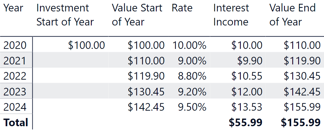
This scenario is straightforward using Excel, because you can simply take the value of the previous year (which is typically in the previous row) as the starting value for the next year to compute the next year’s interest income.
Implementing compound interest in DAX
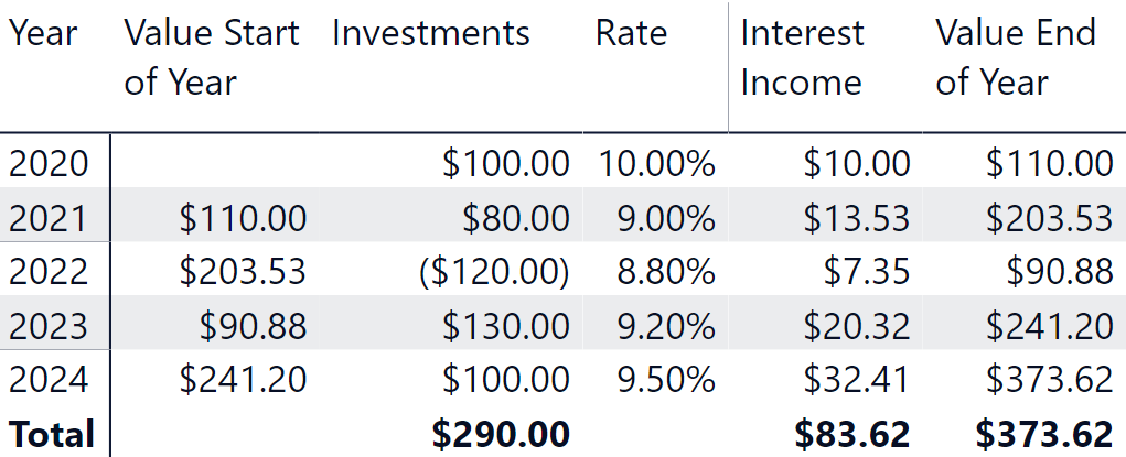
Performing the calculation of compound interest in DAX is challenging, because there is no way to reference the result value in the previous year as we can easily do in Excel. Moreover, in a real data model it is possible that incremental investments are made throughout the holding period. Accordingly, a report could look like the following scenario where an incremental investment is added on the first day of each year over the five-year period (different investment dates during each year would require a different calculation).
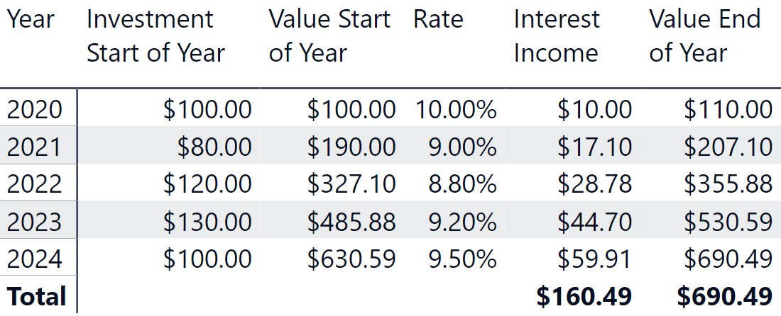
In this case, the value at the end of Year 2 is computed as the sum of $110.00 (value at the end of Year 1) and $80.00 (the value invested on day one of Year 2) increased by 9.0% (the corresponding interest rate for the period).
The sample model we are using for this demo is the following.
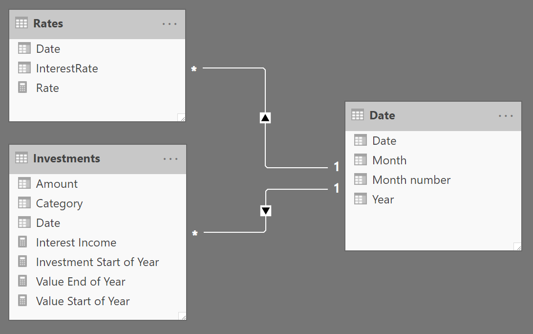
The Investments table contains one row for each investment made over the years, whereas the Rates table contains the different interest rates on a yearly basis. Date is just a simple calendar table.
The main idea to solve the scenario is to split the larger problem into simpler problems. Focus on a year, for example 2022. In 2022 there is an investment of $120. Additionally, in 2022, there are also investments made earlier in 2020 and 2021. Each of these investments has been active for a different number of years: the $100 invested in 2020 have been active for 2 years in 2022, while the $80 invested in 2021 have only been active for one year in 2022.
If we focus on a couple of years – the beginning year and the end year of the investment – the calculation is straightforward: it is enough to multiply the investment amount by (1+interest rate) for every year when the investment is active. This produces the interests gained by the investment over the years when it is active.
With that in mind, the formula to compute the Value End of Year measure can be written as follows, also using the PRODUCTX function:
Value End of Year :=
VAR SelectedYear =
    SELECTEDVALUE (
        'Date'[Year],         -- Find the current year in the report
        MAX ( 'Date'[Year] )  -- default to the last year available
    )
VAR PreviousYears =           -- PreviousYears contains the
    FILTER (                  -- years BEFORE the current one
        ALL ( 'Date'[Year] ),
        'Date'[Year] <= SelectedYear
    )
VAR PreviousInvestments =     -- PreviousInvestments contains
    ADDCOLUMNS (              -- the amount of all the investments
        PreviousYears,        -- made in previous years
        "@InvestedAmt", CALCULATE (
            SUM ( Investments[Amount] )
        )
    )
VAR Result =                  -- For each previous investment
    SUMX (                    -- calculate the compound interest
        PreviousInvestments,  -- over the years and sum the results
        VAR InvestmentYear = 'Date'[Year]
        VAR InvestmentAmt = [@InvestedAmt]
        VAR YearsRateActive =
            FILTER (
                ALL ( Rates ),
                VAR YearRate = YEAR ( Rates[Date] )
                RETURN
                    YearRate >= InvestmentYear
                    && YearRate <= SelectedYear
            )
        VAR CompundInterestRateForInvestment =
            PRODUCTX (
                YearsRateActive,
                1 + Rates[InterestRate]
            )
        RETURN
            InvestmentAmt * CompundInterestRateForInvestment
    )
RETURN
    Result
Although quite long, the formula should be fast enough in most scenarios. Indeed, its complexity does not depend on the size of the Investments table, because that table is scanned only once to perform the grouping by year while computing the PreviousInvestments variable.
The speed of the measure depends solely on the number of years: PreviousInvestments contains one row per year; For each of these years, the formula performs an iteration for all the years up to the selected date.
Therefore, the complexity is around N squared, where N is the number of years of the investment – in real-world scenarios, it should perform well. This approach is possible because the investment is made on the first day of each year – a more complex calculation is required if investment dates are different, but the principle is similar and the calculation over the years should be made at the year level in order to be efficient.
Anyway, the interesting part of this formula is not in its performance. The most relevant detail is that in order to solve the scenario, you need to rethink the algorithm. Trying to solve the formula by thinking in an iterative way – computing the value one year after the other – does not work well in DAX. Rethinking it in terms of evaluating the current value of each investment provides a straight path to the solution that is also more efficient.
Measure optimization for investments made on arbitrary dates
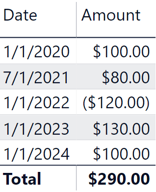
The previous calculation is valid assuming that each investment is made on the first day of each year. If you have a more complex scenario where each investment can have a different date, then you can reuse the previous logic by assuming that the amount you have at the beginning of each year is the amount of the investments made in the previous year added to the interest income at the end of the previous year. This approach also handles capital expenditure reductions, which are recorded as negative transactions in the Investments table. The following screenshot shows an additional investment of $80.00 made on July 1, 2021 and a disinvestment of $120.00 made on January 1, 2022.
The following screenshot shows the expected result.
There are several approaches we can use to implement this solution. A simple one could be to create a measure to compute at the end of each year, the accrued amount of the investments made in that year, and then reuse the measure using the logic of the previous formula. However, this approach results in a query plan with nested iterators that are not ideal in DAX. Therefore, we implemented a different approach that guarantees a better query plan – though this requires a single, more verbose measure.
The following implementation of the Value End of Year measure calculates the sum of the investments at the day level only once. Most of the calculation takes place in the formula engine. However, because the complexity is around D + (N squared) where D is the number of days with investments and N is the number of years, we experienced much better performance with this verbose approach:
Value End of Year :=
VAR SelectedYear =
    SELECTEDVALUE (
        'Date'[Year],         -- Find the current year in the report
        MAX ( 'Date'[Year] )  -- default to the last year available
    )
VAR YearlyInterestRates =
    ADDCOLUMNS (
        CALCULATETABLE (
            ADDCOLUMNS (
                SUMMARIZE (
                    Rates,
                    'Date'[Year]
                ),
                "@InterestRate", CALCULATE (
                    SELECTEDVALUE ( Rates[InterestRate] )
                )
            ),
            REMOVEFILTERS ( 'Date' )
        ),
        "@DailyRate",
            VAR DaysInYear =
                CALCULATE ( COUNTROWS ( 'Date' ) )
            VAR DailyRate =
                [@InterestRate] / DaysInYear
            RETURN
                DailyRate
    )
VAR LastDateInReport =
    CALCULATE (
        MAX ( 'Date'[Date] ),
        ALLSELECTED ( 'Date' )
    )
VAR InvestmentsByDate =
    CALCULATETABLE (
        ADDCOLUMNS (
            SUMMARIZE (
                Investments,
                'Date'[Date],
                'Date'[Year]
            ),
            "@InvestmentAtDate",
                CALCULATE ( SUM ( Investments[Amount] ) )
        ),
        'Date'[Date] <= LastDateInReport
    )
VAR InvestmentsByDateWithRates =
    NATURALLEFTOUTERJOIN (
        InvestmentsByDate,
        YearlyInterestRates
    )
VAR PreviousYears =           -- PreviousYears contains the
    SELECTCOLUMNS (           -- years INCLUDING the current one
        FILTER (
            YearlyInterestRates,
            'Date'[Year] <= SelectedYear
        ),
        "@Year", 'Date'[Year]
    )
VAR PreviousInvestments =     -- PreviousInvestments contains
    ADDCOLUMNS (              -- for each year the amount of
        PreviousYears,        -- all the investments made in the
        "@AccruedAmt",        -- previous year with interest applied
            VAR CurrentYear = [@Year]
            VAR StartOfNextYear = DATE ( CurrentYear + 1, 1, 1 )
            VAR InvestmentsInCurrentYear =
                FILTER (
                    InvestmentsByDateWithRates,
                    'Date'[Year] = CurrentYear
                )
            VAR AccruedAmount =  -- For each investment within the year
                SUMX (           -- sum the amount and accrued interest
                    InvestmentsInCurrentYear,
                    VAR InvestedAmount = [@InvestmentAtDate]
                    VAR DaysInvestment =
                        StartOfNextYear - 'Date'[Date]
                    VAR EffectiveRate =
                        [@DailyRate] * DaysInvestment
                    VAR AccruedInterest =
                        InvestedAmount * EffectiveRate
                    VAR Result =
                        InvestedAmount + AccruedInterest
                    RETURN
                        Result
                )
            RETURN
                AccruedAmount
    )
VAR Result =                  -- For each previous investment
    SUMX (                    -- calculate the compound interest
        PreviousInvestments,  -- over the years and sum the results
        VAR InvestmentYear = [@Year]
        VAR InvestmentAmt = [@AccruedAmt]
        VAR YearsRateActive =
            FILTER (
                YearlyInterestRates,
                'Date'[Year] > InvestmentYear
                    && 'Date'[Year] <= SelectedYear
            )
        VAR CompundInterestRateForInvestment =
            PRODUCTX (                     -- Compute the compound
                YearsRateActive,           -- interest for the
                1 + [@InterestRate]        -- previous years
            )                              -- or returns 1 if there
            + ISEMPTY ( YearsRateActive )  -- are no previous years
        RETURN
            InvestmentAmt * CompundInterestRateForInvestment
    )
RETURN
    Result
Adapting the measure to different granularities
The previous measure only works for a report at the year granularity. This also guarantees a better optimization. If the report needs to be available at different granularities such as quarter and month, the measure is more complex because it must compute the accrued interest on the last day of the period selected. The following is an example of the desired report.
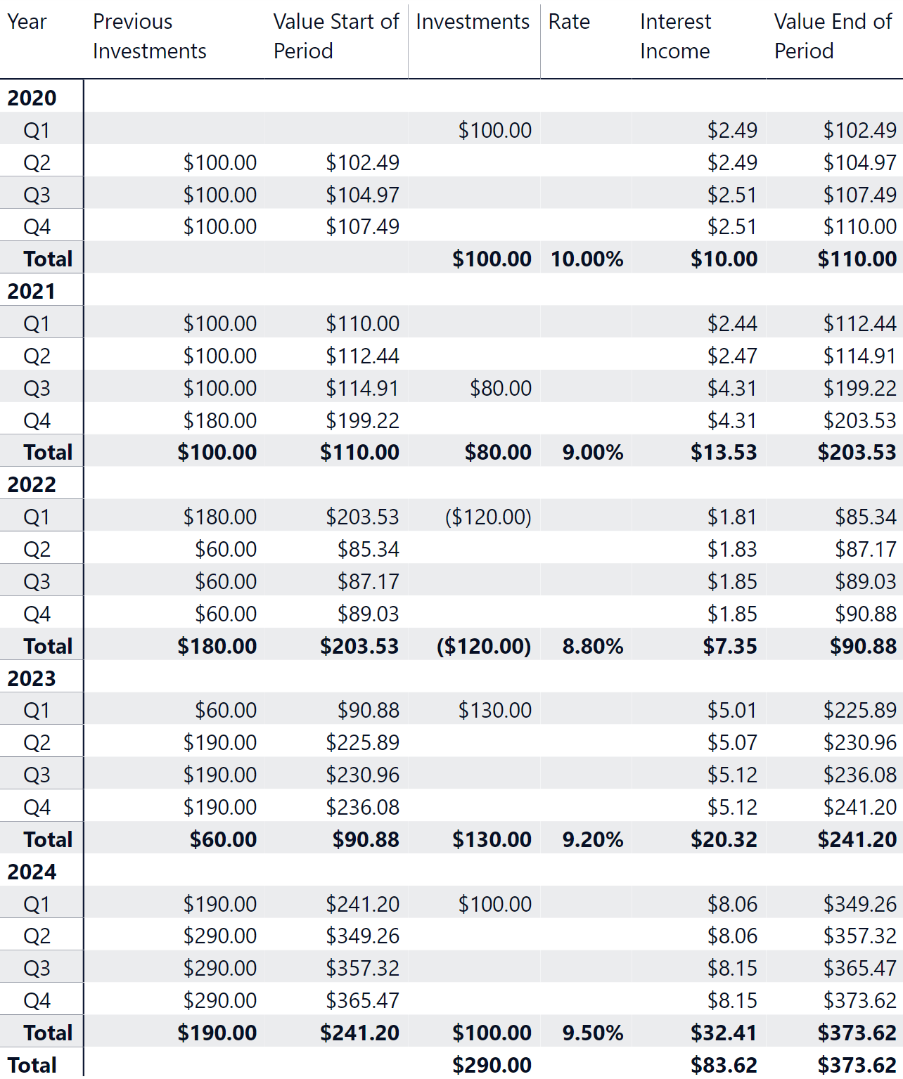
The formula used to produce this report is longer and slower. We suggest only resorting to this approach when absolutely necessary, because it can produce slower reports:
Value End of Period :=
VAR LastDateSelected =
    MAX ( 'Date'[Date] )
VAR LastYearSelected =
    MAX ( 'Date'[Year] )
VAR YearlyInterestRates =
    ADDCOLUMNS (
        CALCULATETABLE (
            ADDCOLUMNS (
                SUMMARIZE (
                    Rates,
                    'Date'[Year]
                ),
                "@InterestRate", CALCULATE (
                    SELECTEDVALUE ( Rates[InterestRate] )
                )
            ),
            REMOVEFILTERS ( 'Date' )
        ),
        "@DailyRate",
            VAR CurrentYear = 'Date'[Year]
            VAR DaysInYear =
                CALCULATE (
                    COUNTROWS ( 'Date' ),
                    REMOVEFILTERS ( 'Date' ),
                    'Date'[Year] = CurrentYear
                )
            VAR DailyRate =
                DIVIDE ( [@InterestRate], DaysInYear )
            RETURN
                DailyRate
    )
VAR LastDateInReport =
    CALCULATE (
        MAX ( 'Date'[Date] ),
        ALLSELECTED ( 'Date' )
    )
VAR InvestmentsByDate =
    CALCULATETABLE (
        ADDCOLUMNS (
            SUMMARIZE (
                Investments,
                'Date'[Date],
                'Date'[Year]
            ),
            "@InvestmentAtDate",
                CALCULATE ( SUM ( Investments[Amount] ) )
        ),
        'Date'[Date] <= LastDateInReport
    )
VAR InvestmentsByDateWithRates =
    NATURALLEFTOUTERJOIN (
        InvestmentsByDate,
        YearlyInterestRates
    )
VAR PreviousYears =           -- PreviousYears contains the
    SELECTCOLUMNS (           -- years INCLUDING the current one
        FILTER (
            YearlyInterestRates,
            'Date'[Year] < LastYearSelected
        ),
        "@Year", 'Date'[Year]
    )
VAR PreviousInvestments =     -- PreviousInvestments contains
    ADDCOLUMNS (              -- for each year the amount of
        PreviousYears,        -- all the investments made in the
        "@AccruedAmt",        -- previous year with interest applied
            VAR CurrentYear = [@Year]
            VAR StartOfNextYear = DATE ( CurrentYear + 1, 1, 1 )
            VAR InvestmentsInCurrentYear =
                FILTER (
                    InvestmentsByDateWithRates,
                    'Date'[Year] = CurrentYear
                )
            VAR AccruedAmount =  -- For each investment within the year
                SUMX (           -- sum the amount and accrued interest
                    InvestmentsInCurrentYear,
                    VAR InvestedAmount = [@InvestmentAtDate]
                    VAR DaysInvestment =
                        StartOfNextYear - 'Date'[Date]
                    VAR EffectiveRate =
                        [@DailyRate] * DaysInvestment
                    VAR AccruedInterest =
                        InvestedAmount * EffectiveRate
                    VAR Result =
                        InvestedAmount + AccruedInterest
                    RETURN
                        Result
                )
            RETURN
                AccruedAmount
    )
VAR FilterLastYearInvestments =
    FILTER (
        InvestmentsByDateWithRates,
        'Date'[Year] = LastYearSelected
    )
VAR LastYearInvestments =
    SUMX (
        FILTER (
            FilterLastYearInvestments,
            'Date'[Date] <= LastDateSelected
        ),
        VAR InvestedAmount = [@InvestmentAtDate]
        VAR DaysInvestment =
            LastDateSelected - 'Date'[Date] + 1
        VAR EffectiveRate =
            [@DailyRate] * DaysInvestment
        VAR AccruedInterest =
            InvestedAmount * EffectiveRate
        VAR Result =
            InvestedAmount + AccruedInterest
        RETURN
            Result
    )
VAR DaysLastYear =
    LastDateSelected - DATE ( LastYearSelected, 1, 1 ) + 1
VAR ValuePreviousInvestments = -- For each previous investment
    SUMX (                     -- calculate the compound interest
        PreviousInvestments,   -- over the years and sum the results
        VAR InvestmentYear = [@Year]
        VAR InvestmentAmt = [@AccruedAmt]
        VAR YearsRateActive =
            FILTER (
                YearlyInterestRates,
                'Date'[Year] > InvestmentYear
                    && 'Date'[Year] <= LastYearSelected
            )
        VAR CompundInterestRateForInvestment =
            PRODUCTX (                     -- Compute the compound
                YearsRateActive,           -- interest for the previous years
                VAR YearRate = 'Date'[Year]
                VAR InterestPreviousYears =
                    [@InterestRate] * (YearRate <> LastYearSelected)
                VAR InterestLastYear =
                    [@DailyRate] * DaysLastYear * (YearRate = LastYearSelected)
                 VAR Result =
                    1 + InterestPreviousYears + InterestLastYear
                RETURN
                    Result
            )                              -- or returns 1 if there
            + ISEMPTY ( YearsRateActive )  -- are no previous years
        VAR FinalInvestmentValue =
            InvestmentAmt * CompundInterestRateForInvestment
        RETURN FinalInvestmentValue
    )
VAR Result =
    ValuePreviousInvestments + LastYearInvestments
RETURN
    Result
Conclusion
The first part of this article presented the overall concepts of dealing with compound interest. We then presented an efficient first DAX approach in computing the compound interest for incremental investments made throughout the holding period. In order to achieve high performance, we moved the calculation logic to the year level. This required an assumption that all investments are made on the first day of each year exclusively.
Later on in the article, we show more complete calculations where every investment can be made at any time and the report can have different granularities. The fundamental idea is the same: compound interest is always calculated at the year level, whereas the value of each investment at the end of the first year is computed with a day granularity. This approach is more verbose, but way more efficient from a computational point of view.
Special thanks to our friend Rick Scanlon, a partner at Innovation Endeavors who helped us write out the definition of compound interest and reviewed the business logic presented in this article.
Calculates the future value of an investment based on a constant interest rate. You can use FV with either periodic, constant payments, or a single lump sum payment.
FV ( <Rate>, <Nper>, <Pmt> [, <Pv>] [, <Type>] )
calculates the present value of a loan or an investment, based on a constant interest rate. You can use PV with either periodic, constant payments (such as a mortgage or other loan), or a future value that’s your investment goal.
PV ( <Rate>, <Nper>, <Pmt> [, <Fv>] [, <Type>] )
Returns the product of an expression values in a table.
PRODUCTX ( <Table>, <Expression> )