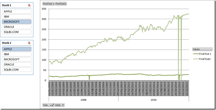
In a previous post, I have used a stock exchange scenario to speak about how to compute moving averages in a complex scenario. Playing with the same scenario, I felt the need to compare two stocks on the same chart, choosing the stock names with a slicer. As always, a picture is worth a thousand words, the final result I want to achieve is something like this, where I am comparing Microsoft over Apple during the last 10 years.
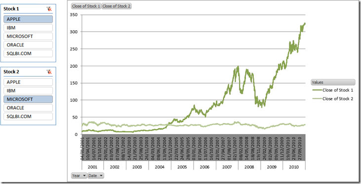
It is clear that I am not going to comment in any way why traders seem to prefer buying Apple instead of Microsoft… this would be the task of a trader and I am only a BI guy. ![]()
What makes this scenario interesting is that there are two values in the chart (Close of Stock 1 and 2) and their values will be determined by a slicer. I want to use the same chart to compare, for example, Oracle vs SQLBI.COM. Thus, the value of the measure need to be determined dynamically, depending on the value of the slicer. This is a pretty common example of a slicer used to “inject” parameters inside DAX formulas, i.e. the DAX formula will compute different values depending on parameters that the user can select with filters, slicers or any other UI tool.
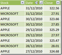
First of all, let us recall briefly the content of our tables: we have a Fixing table, containing the values of the stocks as they change during time, with a granularity at the day level, and a standard calendar table. The Fixing table is very easy:
Now, it should be evident that “Close of Stock 1” cannot be computed as a calculated column, since its value depends on the evaluation context defined by the slicer. Thus, the starting point is a measure. Similarly, the slicers for Stock 1″ and 2 cannot use the Stock column in the Fixing table since their usage will be that of changing the measure behavior, not to filter the fixing table (or, in other words, the filter will be controlled by the DAX formula).
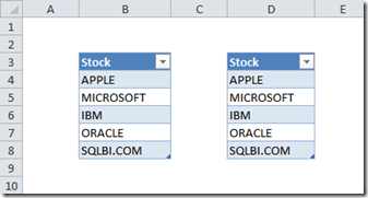
Thus, the first step is to create two Excel tables that will be used as the sources for the slicers. This is pretty easy: just create two Excel tables like the ones shown below, link them in PowerPivot and call them Stock1 and Stock2. The first part is gone easily.
Then, in order to define the value of “Close of Stock 1”, we need to:
- Check if the slicer for Stock1 filters one stock (the user might remove the filter and, in this case, the value of the measure is undefined)
- Compute the value of the measure based on the stock name selected in the Stock1 slicer
This is pretty easy to accomplish, using this formula:
=IF (
    COUNTROWS (VALUES (Stock1[Stock 1])) <> 1,
    BLANK (),
    CALCULATE (
        AVERAGE (Fixing[Close]),
        Fixing[Stock] = VALUES (Stock1[Stock 1])
    )
)
The key of this formula is in the definition of the filter context under which CALCULATE computes the AVERAGE of Fixing[Close]. We ask for a filter context where the Fixing[Stock] column shows only the values for the stock in Stock1[Stock 1], which is the name of the stock selected in the slicer. Moreover, we know that the VALUES function will return exactly one row, since we test if in the preceding IF. As always, it is easier to read than to create, take your time to understand it well. ![]()
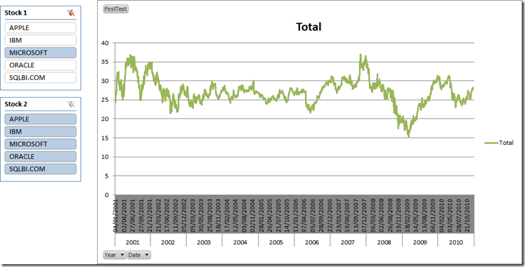
If you define this formula and create a PivotChart putting years and dates on the Axis, you get this first nice result:
Clearly, you can define a new measure tied to the Stock2 table, add it to the chart and you will get this result which does not look as pretty as before (in the example, I have filtered only the last two years to make the issue more evident):
You can see that there are points in time (near November 2011 and July 2010) where both stocks present a spike down to zero. The interesting part is the fact that these spikes do not appear when only one stock is added to the chart, they appear only when we put two stocks on the same chart.
The reason for this behavior is that in my set of data, there are some dates where the value of one stock has not been recorded, for whatever reason. When only one stock is in the chart, those dates are removed from the graph. Nevertheless, when both stocks are present on the same chart, if it happens that the value of one of the two stocks is present, then that date will be present in the chart too. Now, for that date, the value of the other stock yields zero, resulting in the annoying issue we are facing on this chart: i.e. spikes down to zero when only one of the two stocks has been recorded.
We could (and should) remove the problem updating the original table, adding interpolated values where they are not present. Nevertheless, since this is a post about DAX, we’d better resolve the issue using DAX. The idea is that, if Stock2 is not present for a period of time, we should not return any value for Stock1 too. The contrary holds true: if Stock1 is not present, then Stock2 should not return any value. Thus, at the end both Stock1 and Stock2 will return values only for dates where both are present.
The formula, for Close of Stock 1 is the following:
=IF (
    COUNTROWS (VALUES (Stock1[Stock 1])) <> 1 || COUNTROWS (VALUES (Stock2[Stock 2])) <> 1,
    BLANK (),
IF (
        ISBLANK (
            CALCULATE (
                AVERAGE (Fixing[Close]),
                Fixing[Stock] = VALUES (Stock2[Stock 2])
            )
        ),
        BLANK (),
        CALCULATE (
            AVERAGE (Fixing[Close]),
            Fixing[Stock] = VALUES (Stock1[Stock 1])
        )
    )
)
If both slicers select one value each then, if Stock2 is present, then calculate Stock1 otherwise return BLANK. The formula for Stock2 is very similar, with some 1 and 2 interchanged. Updating the formulas is enough to get the nice result of the first chart, which was our final goal.
Clearly, the very same technique can be used to add more interesting measures, like Bollinger Bands, moving averages or, with a bit more effort, turn PowerPivot in a complete trading system that suggests when to buy or to sell a stock. This is left as an interesting exercise to the reader. ![]()
This is just another example of what PowerPivot can do for your reporting needs. If you want to touch the real Karma of PowerPivot, don’t miss the opportunity to follow one of the workshops I and Marco Russo are bringing all over Europe in the next few months.
You can find more info on www.powerpivotworkshop.com. Hope to see you there!
Checks whether a condition is met, and returns one value if TRUE, and another value if FALSE.
IF ( <LogicalTest>, <ResultIfTrue> [, <ResultIfFalse>] )
Counts the number of rows in a table.
COUNTROWS ( [<Table>] )
When a column name is given, returns a single-column table of unique values. When a table name is given, returns a table with the same columns and all the rows of the table (including duplicates) with the additional blank row caused by an invalid relationship if present.
VALUES ( <TableNameOrColumnName> )
Returns a blank.
BLANK ( )
Evaluates an expression in a context modified by filters.
CALCULATE ( <Expression> [, <Filter> [, <Filter> [, … ] ] ] )
Returns the average (arithmetic mean) of all the numbers in a column.
AVERAGE ( <ColumnName> )
Checks whether a value is blank, and returns TRUE or FALSE.
ISBLANK ( <Value> )