The importance of star schemas in Power BI

A common question among data modeling newbies is whether it is better to use a completely flattened data model with only one table, or to invest time in building a proper star schema (you can find a description of star schemas in Introduction to Data Modeling). As coined by Koen Verbeeck, the motto of a seasoned modeler should be “Star Schema all The Things!”

The goal is to demonstrate that a report using a flattened table returns inaccurate numbers, whereas using a star schema turns it into a sound analytical system.

The data model to analyze is simple. A company owns four beauty salons: two hair salons and two nail salons. Patrons visit the salons and provide relevant information, like their gender and job. You need to build a simple report to analyze the number of visits, sliced by gender and job for one salon. In the same report, you want to compare the visits of the currently selected salon against the group it belongs to. In other words, the question to answer is: how is the distribution of job and gender among patrons of a given salon compared with the average of all the salons of the same type?

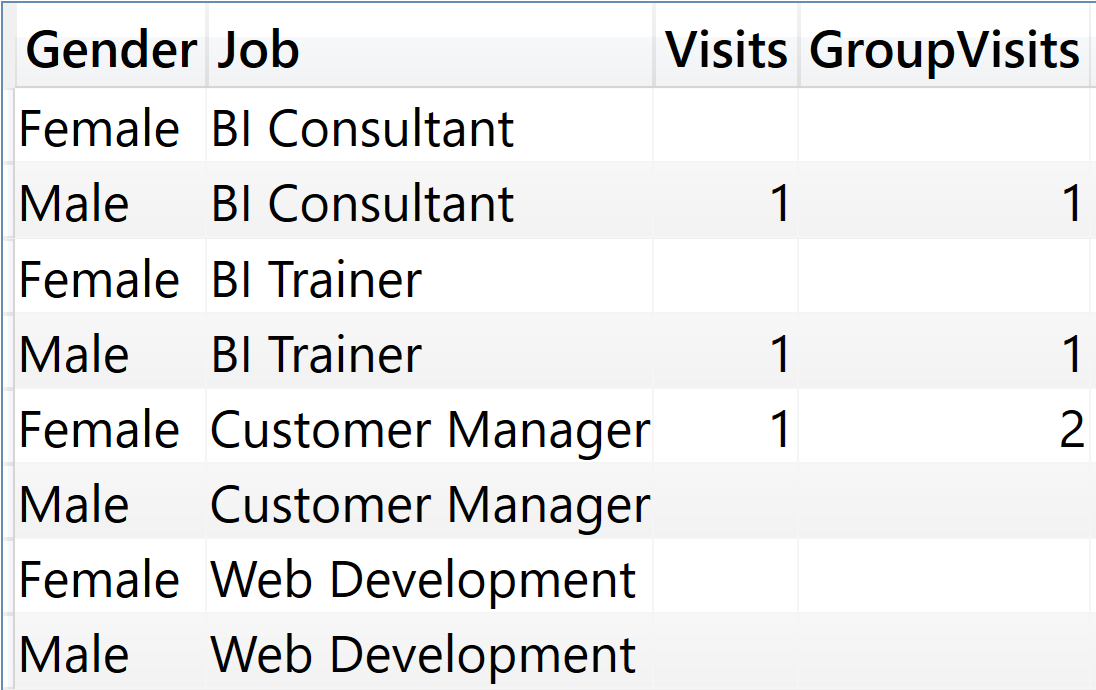
The source is a single table, already containing all the relevant information.

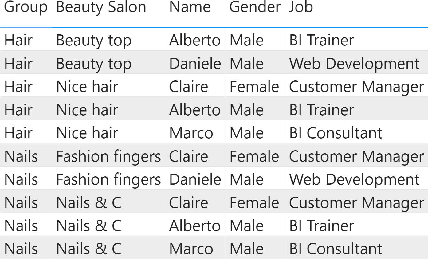
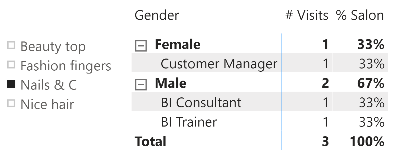
Because the table does not contain any keys and all the information is already there, it looks like there is no need to build a data model on top of it – one table is enough. Indeed, a report with the number of visits along with their percentage produces the correct results.

In the report, we use these measures:

# Visits := COUNTROWS ( 'Visits' )

% Salon := 
VAR NumOfVisits = [# Visits]
VAR NumOfAllVisitsSameSalon = 
    CALCULATE (
        [# Visits],
        REMOVEFILTERS ( 'Visits' ),
        VALUES ( 'Visits'[Beauty Salon] )
    )
VAR Result = DIVIDE ( NumOfVisits, NumOfAllVisitsSameSalon )
RETURN Result

% Salon achieves its goal by dividing the number of visits by the total number of visits at that salon, regardless of any other filter.

The second step proves to be a lot more challenging. We want to show the distribution of genders and jobs across all the salons of the same group (hair vs. nails). The first step would be to compute how many visits there have been in the group that the current salon belongs to. The following measure does not compute the right numbers, even though it looks perfectly correct:

# Group Visits := 
CALCULATE( 
    [# Visits], 
    REMOVEFILTERS ( 'Visits'[Beauty Salon] ),
    VALUES ( 'Visits'[Group] )
)

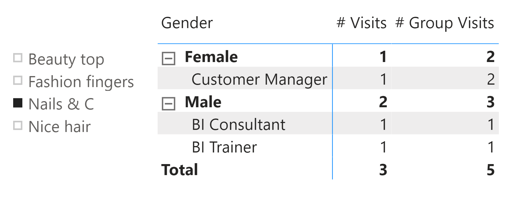
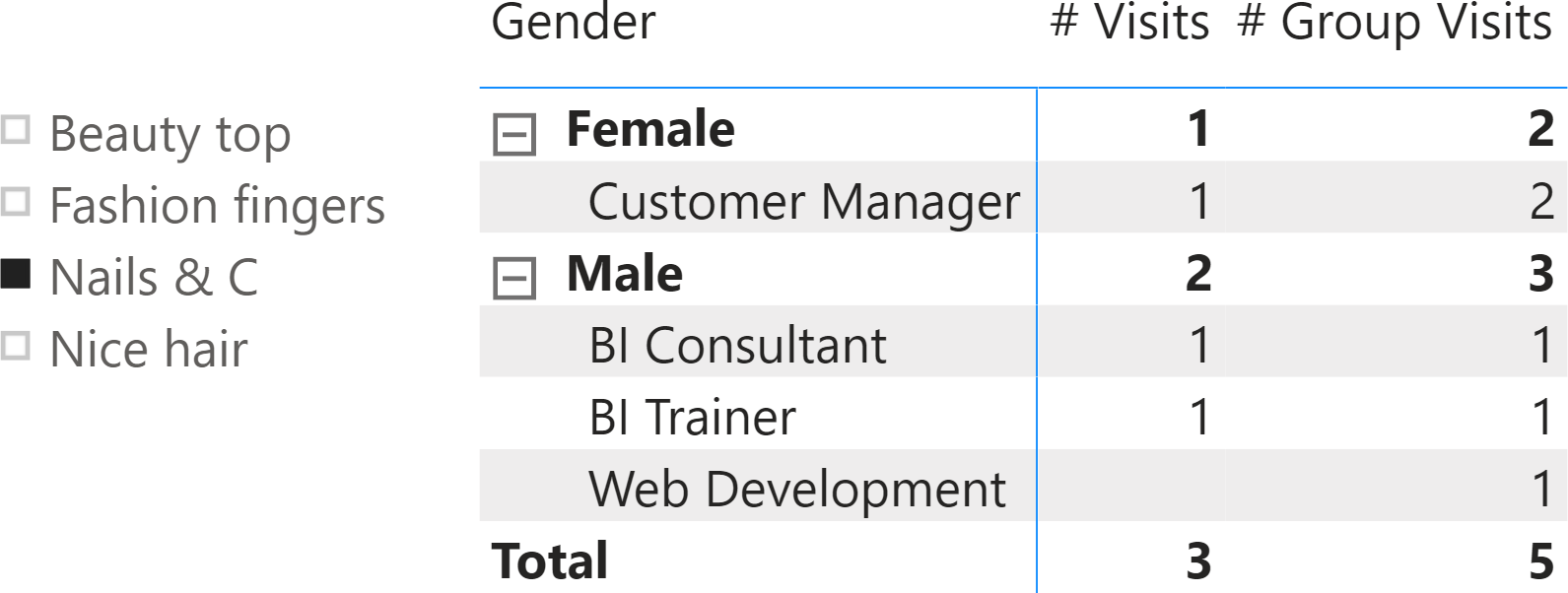
Look at the result:

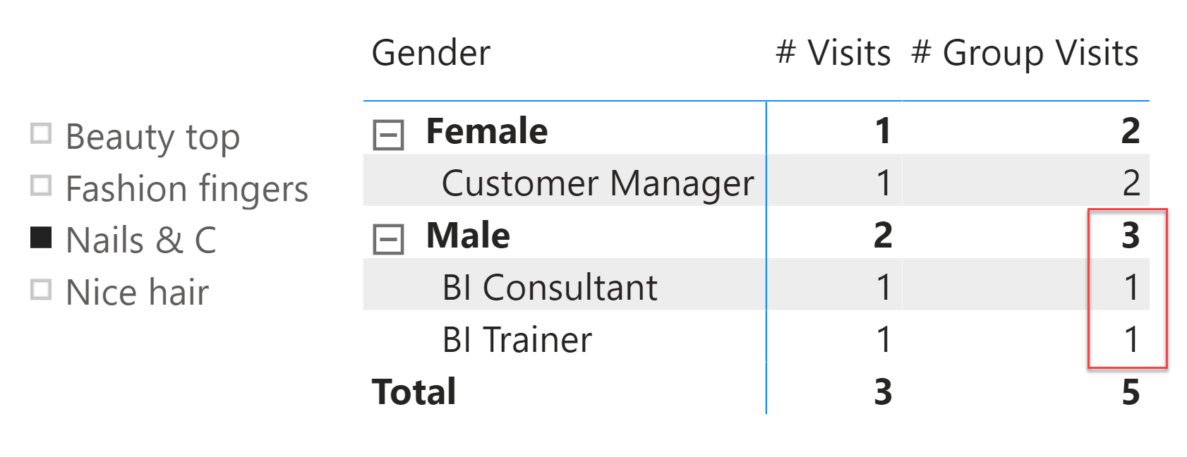
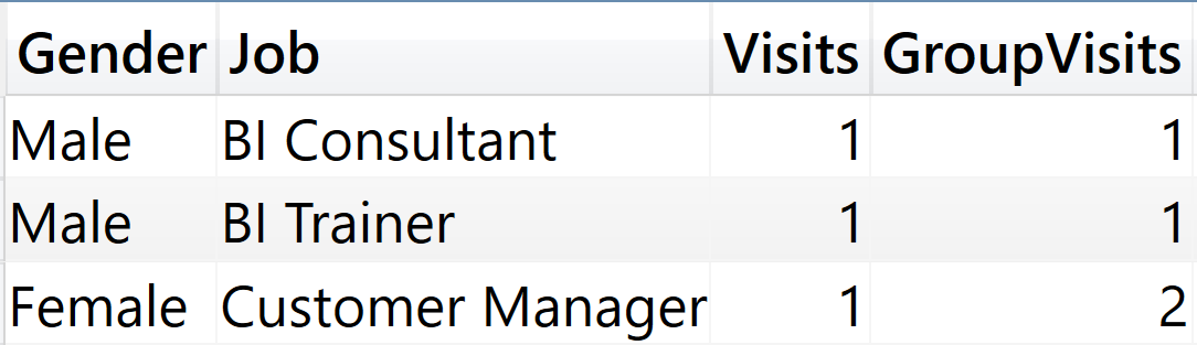
The report is clearly wrong. You can easily check that the totals are fine. There have been three male visits in the Nails group as per the source table displayed previously, but one is not reported in the detail. This example, in its simplicity, is wrong for two reasons.

The first reason is the “auto-exist” behavior – an internal optimization of DAX we described in a previous article. The second reason is the model’s inability to find the relationship between group and salon in the current data model when there are no visits.

When SUMMARIZECOLUMNS scans the table under a filter context with Nails & C for Beauty Salon and Male for Gender, it merges the two filters into one, preventing it from finding the missing Job (Web Development). If you are unfamiliar with this behavior, we strongly suggest having a look at the article mentioned above which goes deeper in explaining the “auto-exist” behavior.

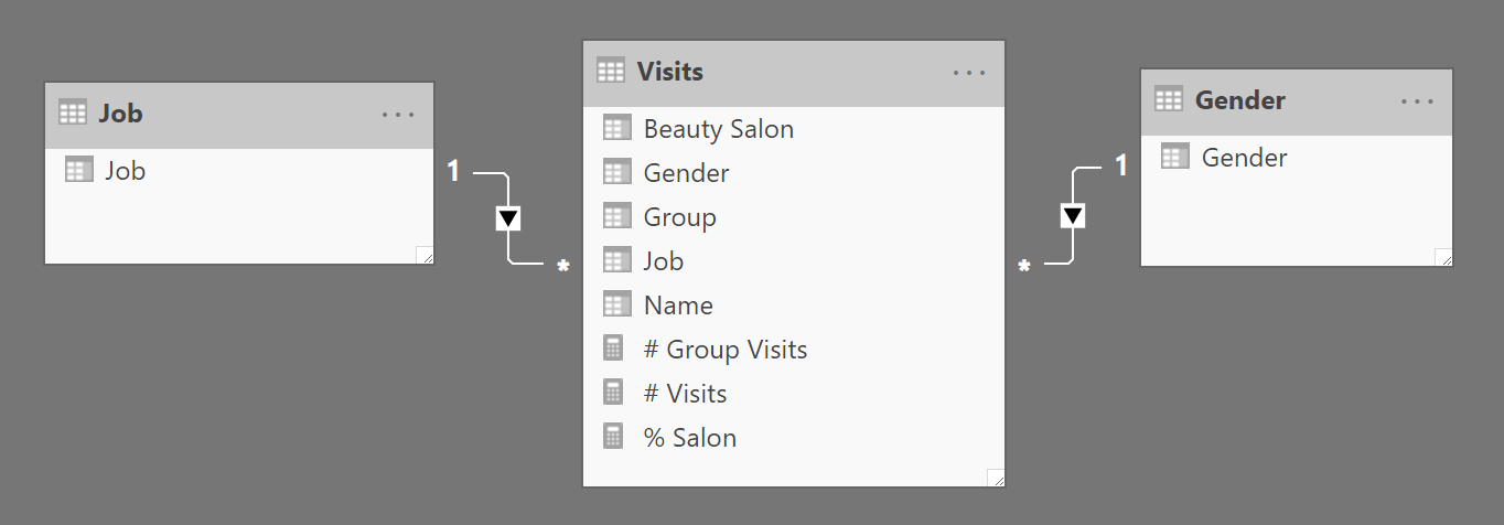
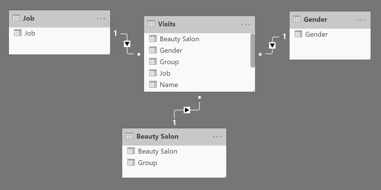
Avoiding the effect of auto-exist is simple: you need to create separate dimensions for gender and job, so that a filter on one dimension does not affect the other dimensions. This simple operation prevents auto-exist from kicking in.

Therefore, a first (required, though not yet final) step in solving the problem is to create two dimensions: one for the gender and one for the job.  The new model looks more like a star schema.

Then, you need to update the matrix slicing by the columns in the dimensions instead of the columns in the fact table. Nevertheless, this is not enough to solve the problem, even though we removed the issue of auto-exist. Indeed, the numbers look the same – still wrong.

In order to make sure that auto-exist is no longer an issue, you can catch the query executed by Power BI through the performance analyzer, clean it up a bit, and here is what it looks like:

DEFINE
    VAR __DS0FilterTable =
        TREATAS ( { "Nails & C" }, 'Visits'[Beauty Salon] )
    VAR __DM3FilterTable =
        TREATAS ( { "Female", "Male" }, 'Gender'[Gender] )
EVALUATE
SUMMARIZECOLUMNS (
    'Gender'[Gender],
    'Job'[Job],
    __DS0FilterTable,
    __DM3FilterTable,
    "Visits", 'Visits'[# Visits],
    "GroupVisits", 'Visits'[# Group Visits]
)

Because SUMMARIZECOLUMNS is grouping and filtering through two separate tables, auto-exist does not kick in. You can easily double-check this by running two slightly modified versions of this query. We first introduce IGNORE on the measures to avoid the removal of blank rows; we then execute the same query grouping first by the dimensions (Gender, Job) and then by the columns in the fact table.

This is the query that groups the dimensions:

DEFINE
    VAR __DS0FilterTable =
        TREATAS ( { "Nails & C" }, 'Visits'[Beauty Salon] )
    VAR __DM3FilterTable =
        TREATAS ( { "Female", "Male" }, 'Gender'[Gender] )
EVALUATE
SUMMARIZECOLUMNS (
    'Gender'[Gender],
    'Job'[Job],
    __DS0FilterTable,
    __DM3FilterTable,
    "Visits", IGNORE ( 'Visits'[# Visits] ),
    "GroupVisits", IGNORE ( 'Visits'[# Group Visits] )
)

The result shows that all the combinations of gender and job are returned, despite the fact that many are blank.

This is the query that groups the columns from the fact table:

DEFINE
    VAR __DS0FilterTable =
        TREATAS ( { "Nails & C" }, 'Visits'[Beauty Salon] )
    VAR __DM3FilterTable =
        TREATAS ( { "Female", "Male" }, 'Gender'[Gender] )
EVALUATE
SUMMARIZECOLUMNS (
    'Visits'[Gender],
    'Visits'[Job],
    __DS0FilterTable,
    __DM3FilterTable,
    "Visits", IGNORE ( 'Visits'[# Visits] ),
    "GroupVisits", IGNORE ( 'Visits'[# Group Visits] )
)

As you see, the result does not include pairs of gender and job that did not visit Nails & C.

Therefore, the first step was successful and auto-exist is no longer in action here. We already knew this step was required, but this is still not enough to address the issue. The problem is a bit more subtle to find, even though the nature of the problem is very close to an auto-exist.

The missing line in our report is (Male, Web Development). Because we have two dimensions, Job and Gender, we know that SUMMARIZECOLUMNS actually computes the value for this combination. Nevertheless, it comes out as a blank. We need to investigate further to determine the reason.

For the combination Gender=Male, Job=Web Development, DAX computes this measure:

# Group Visits := 
CALCULATE( 
    [# Visits], 
    REMOVEFILTERS ( 'Visits'[Beauty Salon] ),
    VALUES ( 'Visits'[Group] )
)

Therefore, we can expand the full expression, to better understand what is going on:

EVALUATE
{
    CALCULATE (
        CALCULATE (
            [# Visits],
            REMOVEFILTERS ( 'Visits'[Beauty Salon] ),
            VALUES ( 'Visits'[Group] )
        ),
        'Visits'[Beauty Salon] = "Nails & C",
        'Gender'[Gender] = "Male",
        'Job'[Job] = "Web development"
    )
}

The inner CALCULATE evaluates the VALUES function in the filter context defined by the outer CALCULATE. Because there are no male web developers visiting Nails & C., VALUES ( ‘Visits'[Group] ) returns an empty table, not a table with the group the salon belongs to.  Therefore, the measure returns blank.

Though this behavior is very close to auto-exist, this time the fault is entirely ours. DAX has no part in the calculation being inaccurate. When the set of filters in the filter context produces an empty result, there is no way of discovering which group the current salon belongs to, because there are no rows in the Visits table telling us this information. In other words, we are relying on the fact table to tell us which group a salon belongs to. In the absence of visits, the information is not available.

Understanding the problem is much harder than finding the solution. To avoid the issue we need to define a data structure containing salons and their respective group. This table cannot be the Visits table, which can be filtered by the report; it needs to be a dedicated dimension. Therefore, the final step to solve the scenario is to build a third dimension for the beauty salons with a table named Beauty Salon.

Once the dimension is in place, we use a slicer with the Beauty Salon column of the Beauty Salon table instead of the Beauty Salon column from the Visits table, and then we make a minor correction to the DAX code:

# Group Visits := 
CALCULATE( 
    [# Visits], 
    REMOVEFILTERS ( 'Beauty Salon'[Beauty Salon] ),
    VALUES ( 'Beauty Salon'[Group] )
)

As you see, the REMOVEFILTERS and the VALUES functions operate on the dimension instead of working against the columns in the fact table. The overall logic of the measure remains the same. With this new measure in place, the report now shows the correct results.

Spotting the issue on a model with 10 rows proved to be challenging from the DAX point of view, but it was made easier by the fact that we knew what numbers to expect in the result. Needless to say, it would be absolute hell having to find the issue on a model with millions of rows. This is why expert modelers always follow these rules:

• Use a star schema. Always.
• Hide all the columns in the fact table. Only show measures in the fact table.
• Expose visible attributes only through dimensions.
• Test your formulas on small sets of data that you can master and understand at a glance.

These are golden rules. Expert modelers may decide to override the rules, but they do so with a deep and thorough understanding of what they are dealing with. Inexperienced modelers oftentimes choose to avoid rules. Doing so is exciting, if you want to feel the thrill of wandering into a totally unexplored and dangerous maze of complexity. On the other hand, if you want to deploy a sound model for your customers, then obeying these simple rules is a very good step in the right direction.