The hidden complexity of a daily average in DAX

Computing an average daily sales amount is straightforward: you should iterate over the dates, compute sales for each day, and average the results. An AI assistant can generate DAX code that works in just a few seconds; whether it computes the number you need is a different question.

In this article, we ask AI to generate every measure, function, and validation query. We start with a simple average and test it against more demanding scenarios. Our job is to explain the business requirements, challenge the proposed code, and verify the results. Each test reveals a missing detail from the original request.

The prompts below show a conversation with an AI agent. They describe how to get the DAX code from the AI. They are not a verbatim transcript: a different agent might produce different expressions.

The goal is not to test the assistant or demonstrate complex DAX code. The goal is to show that AI makes it easier to write code. In doing so, it leaves more time for humans to focus on inspecting border cases, refining the formula, and producing better calculations. The very same scenario would be challenging for a human, too.

We start with the following prompt:

Create a measure Average Daily Sales (Selling Days) that computes the average daily sales amount by iterating over Date and computing [Sales Amount]

A plausible answer is the following, although your execution result may differ:

Average Daily Sales (Selling Days) =
AVERAGEX ( 'Date', [Sales Amount] )

The Date table contains one row per day. DAX evaluates Sales Amount for each date visible in the filter context, as it iterates the Date table reference. We can ask the assistant to iterate over the Date[Date] column:

Rewrite the measure to iterate over the distinct values of Date[Date], instead of the entire Date table. Keep the existing blank-handling behavior and explain whether this change affects the denominator in this model.

Average Daily Sales (Selling Days) =
AVERAGEX ( VALUES ( 'Date'[Date] ), [Sales Amount] )

The measure now works on a single-column table, and it seems a bit more efficient. However, both versions have the same issue: AVERAGEX excludes blank results from the average but considers zero as a relevant value. The two different table expressions produce the same behavior and result.

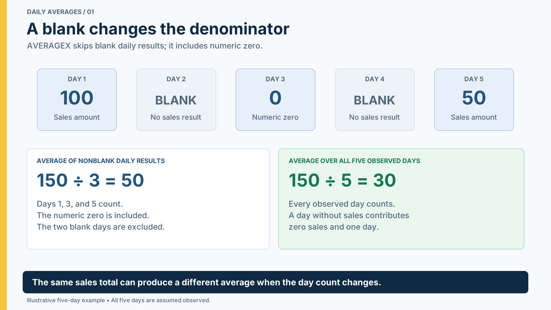
The following figure shows a simple average over five rows, with the two possible calculations. AVERAGEX performs the calculation on the left, and it ignores blanks.

To make the issue more evident, look at the following matrix, where we filtered one color (Brown) and expanded January 2024.

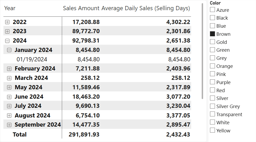
The value shown for January 2024 is the same as 01/19/2024, the only day with sales.

Product filters Sales; therefore, it filters its results, but it does not filter Date through the single-direction relationships. January shows 31 days, but Sales Amount is blank for 30 of them. We can ask AI for a query that makes the denominator visible:

Show me a DAX query for January 2024 that compares all product colors with the color Brown. Return the color, sales amount, the number of dates with a nonblank Sales Amount, and the average over those dates. Use the Sales Amount measure and query-scoped definitions for any additional measures. Do not change the model. Explain why a date without sales is excluded from this average.

The query generated should return a result very similar to the following one.

January 2024	Sales Amount	Days with sales	Average Daily Sales (Selling Days)
All colors	188,419.28	27	6,978.49
Brown	8,454.80	1	8,454.80

In January 2024, total sales are 188,419.28 across 27 days. The first measure returns 6,978.49. January has 31 days, but four have a blank Sales Amount and are excluded from the denominator. For Brown products, things are even worse: only one day has sales. In both cases, the number of considered days is less than 31.

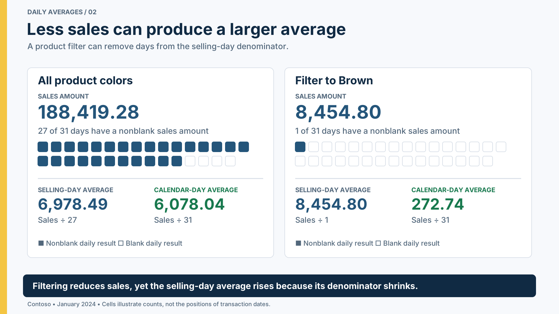
There is no arithmetic error here. The measure computes average sales over days with a non-blank Sales Amount. For this sample, these are the days with sales. If this is the intended business definition, the measure is correct. However, if we want average sales per calendar day, the Brown result should be 8,454.80 divided by 31, or 272.74: the denominator should include days without sales.

To obtain the latter definition, we include an additional requirement in the prompt:

Generate a revised measure named Average Daily Sales (Calendar Days). Divide the total Sales Amount by the number of visible rows in Date, which has one row per day. A product filter must change the amount without removing days from the denominator. Use safe division, preserve a blank amount for now, and do not yet adjust for the beginning or end of the available history.

The generated measure does not have an iterator anymore:

Average Daily Sales (Calendar Days) =
DIVIDE ( [Sales Amount], COUNTROWS ( 'Date' ) )

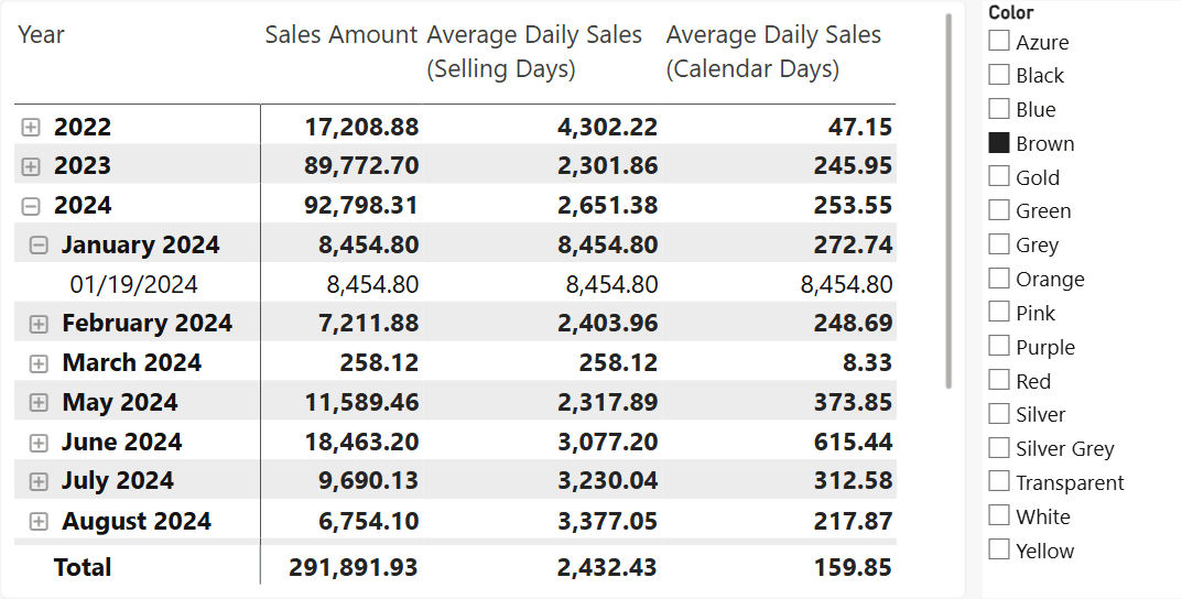
Because Date contains one row per day, COUNTROWS returns the number of visible days. A filter on Product changes the numerator and not the denominator, because Date does not receive filters from other tables. The result now corresponds to the more refined requirements.

Another option would have been to replace blanks with zero inside AVERAGEX. For a period with sales, that would solve the denominator problem, even though the measure generated would be slower.

However, neither approach tells us whether all visible dates should participate in the calculation, in case the available calendar goes beyond the date range for which we have transactions.

To evaluate that condition, we ask AI to inspect the dates with the following prompt:

Generate a DAX query returning one row with the number of Date rows, the minimum and maximum Date[Date], the number of Sales rows, the minimum and maximum Sales[Order Date], the distinct count of order dates, and Sales Amount. Also count blank order dates and distinct order dates missing from Date. Query the model without modifying it. Report the date ranges without assuming that the first and last transaction prove data completeness.

The query shows that the calendar runs from January 1, 2022 through December 31, 2026. The first transaction is on May 21, 2022, and the last is on March 21, 2026.

Field	Result
Date Rows	1,826
First Calendar Date	January 1, 2022
Last Calendar Date	December 31, 2026
Sales Rows	3,996
First Order Date	May 21, 2022
Last Order Date	March 21, 2026
Distinct Order Dates	880
Sales Amount	4,373,105.53
Blank Order Date Rows	0
Distinct Order Dates Missing from Date	0

The calendar in the Date table has months without transactions. Even if we reduce the calendar from May 2022 to March 2026, May 2022 (the first month with sales) contains 11 observed days, and March 2026 (the last month with sales) contains 21. Dividing sales by 31 days in either month understates the average.

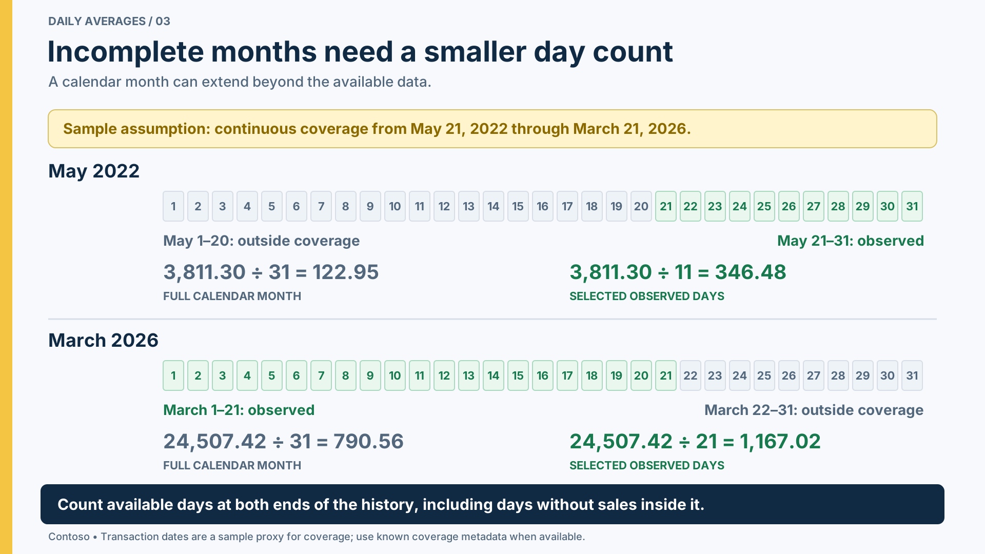
The problem occurs at both ends of the available history. It also affects totals that include dates before or after that history, in case we did not reduce the calendar.

Notice the assumption we just introduced. The first transaction does not prove that data collection started on that date, and the last transaction does not prove that later dates are unavailable. It is possible that there were no sales on other days.

For the following example, we use the first and last transaction dates as the boundaries of a continuous observation period. We consider every date within that period available, including dates without transactions. In a production model, it is better to use exact data-availability dates when transaction dates cannot be used reliably.

Before improving the formula, we can ask AI to challenge the definition:

Review this average daily sales calculation before proposing another formula. Find small examples that distinguish days without sales from days outside the available data. Include product filters, incomplete first and last months, an empty period, nonconsecutive date selections, and totals. State the expected denominator and identify any business rule that the data alone cannot establish.

This is a useful role for AI. Instead of asking only for implementation, we also ask it to find cases that might disprove it. A proposed test becomes useful when we can state its expected result independently and then execute it.

The AI result is a table containing several edge case scenarios that must be carefully inspected and covered by our new rule.

Test	Small example	Expected denominator
Day without sales	Select May 22, 2022, which has no transactions but lies inside coverage.	1 day
Day outside coverage	Select May 20, 2022, before assumed coverage starts.	0 days
Product filter	Select January 2024 and Brown products. Brown has sales on one day, but the entire month is observed.	31 days, not 1
Incomplete first month	Select May 2022. Count May 21–31, including days without sales.	11 days, not 31
Incomplete last month	Select March 2026. Count March 1–21, even though its first transaction is March 3.	21 days, not 31
Observed period without product sales	Select March 2026 and Green products. Green has no sales that month.	21 days
Period entirely outside coverage	Select April 2026. No selected dates fall inside the coverage.	0 days
Empty date selection	Apply a filter that selects no dates.	0 days
Nonconsecutive dates	Select May 21, 22, and 28, 2022. Include the blank sales result on May 22, but exclude unselected dates between them.	3 days, not 8
Nonconsecutive months	Select January and March 2024. February is not selected.	62 days, not 91
Total across unequal periods	Select February and March 2026 together. February contributes 28 days; March contributes 21.	49 days

After analyzing the scenarios, we end up with the following requirements for our average:

• Count the selected dates that fall within the observation period.
• Include days without sales within that period.
• Use the same observation period for every product, customer, and store selection.
• Return zero when there are days observed but no sales for the current selection.
• Return blank when there are no observed days selected.

The difference between zero and blank matters: zero means we observed a time period and found no sales; blank means we want to ignore that period for the average.

A possible mistake would be to compute the first and last sale after removing only the Date filter, because it is incompatible with our requirements. With that approach, a product selection can move the boundaries. In our sample file, the last sale of a Green product is February 12, 2026, whereas other products have sales through March 21, 2026. Selecting Green should not make March unavailable. However, for our requirements, the March average is zero over 21 days observed.

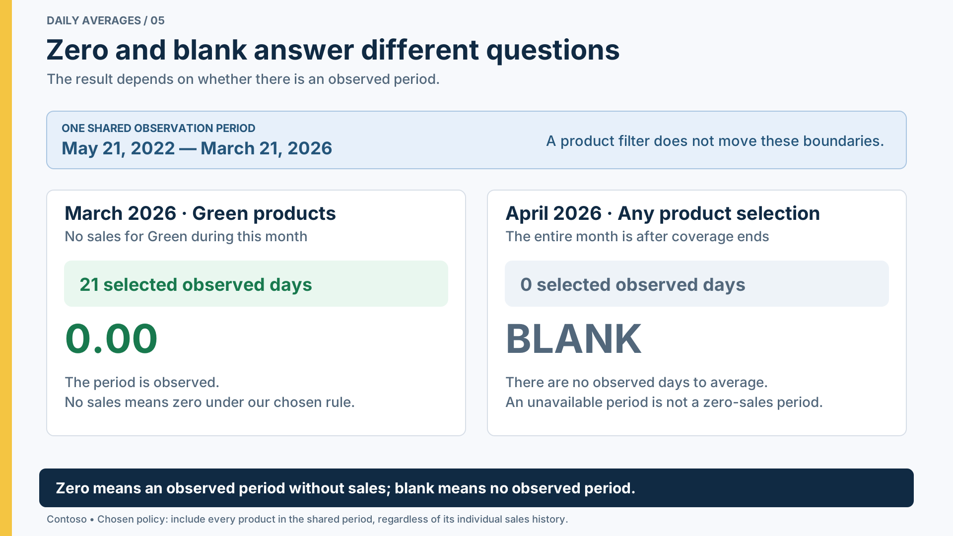
For the same reason, we must not use each month’s first and last transaction as that month’s boundaries. March 2026 has its first transaction on March 3, but March 1 and March 2 are inside the overall observation period, so they must be counted.

We now have enough information to create the request for the complete measure:

Generate a measure named Average Daily Sales using these rules:
– Define one inclusive observation period from the first to the last Sales[Order Date], ignoring all ordinary report filters when finding those boundaries.
– Count only currently visible, nonblank Date[Date] values inside that period.
– Preserve nonconsecutive selections.
– Compute Sales Amount over exactly those dates while preserving the other report filters.
– Include dates without sales in the denominator.
– Return zero for an observed selection without sales, and blank if there are no observed dates or no boundary dates.
– Use variables to make the steps readable.

The resulting code is considerably longer than the first expression we obtained at the beginning of the article:

Average Daily Sales =
VAR FirstObservedDate =
    CALCULATE ( MIN ( Sales[Order Date] ), REMOVEFILTERS () )
VAR LastObservedDate =
    CALCULATE ( MAX ( Sales[Order Date] ), REMOVEFILTERS () )
VAR ObservedDates =
    FILTER (
        VALUES ( 'Date'[Date] ),
        NOT ISBLANK ( 'Date'[Date] )
            && 'Date'[Date] >= FirstObservedDate
            && 'Date'[Date] <= LastObservedDate
    )
VAR NumberOfDays = COUNTROWS ( ObservedDates )
VAR Amount =
    CALCULATE ( [Sales Amount], KEEPFILTERS ( ObservedDates ) )
RETURN
    IF (
        NOT ISBLANK ( FirstObservedDate )
            && NOT ISBLANK ( LastObservedDate )
            && NumberOfDays > 0,
        DIVIDE ( COALESCE ( Amount, 0 ), NumberOfDays )
    )

FirstObservedDate and LastObservedDate are evaluated after removing any report filters. Therefore, a filter on products or months in a matrix row does not move the boundaries. REMOVEFILTERS does not bypass row-level security: the interval is shared within the data visible to the current security context.

ObservedDates starts from VALUES ( ‘Date'[Date] ), which contains the dates visible in the current filter context. FILTER keeps only those dates within the observation period and excludes a possible blank member.

The code considers only the selected dates. For example, if the user selects January and March, the denominator must not include February. If it counted the elapsed days between the first and last selected date, it would include February, which the user could have excluded. The same principle applies to a selection of individual days or weekdays.

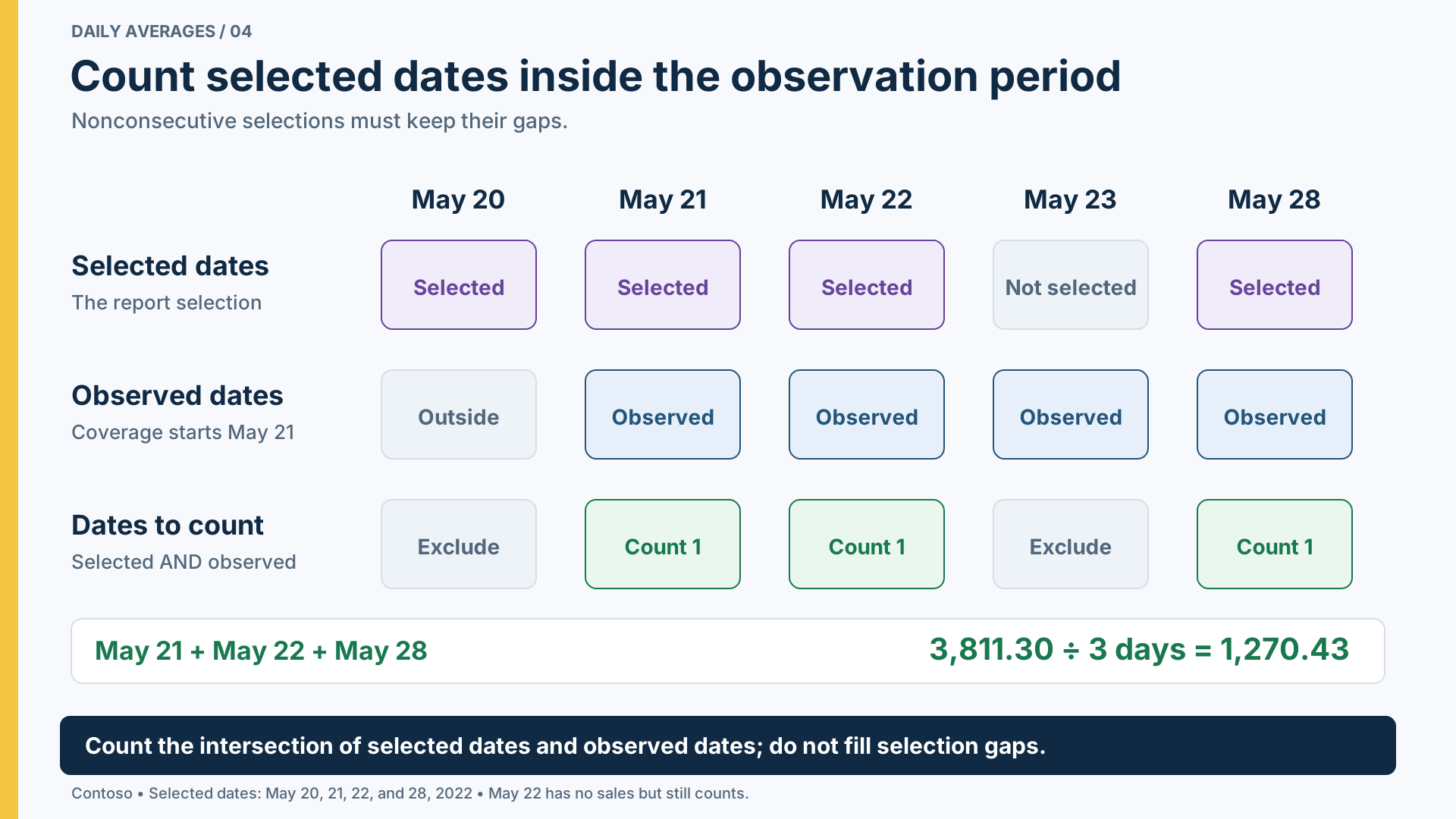
The Average Daily Sales measure then counts ObservedDates and evaluates Sales Amount over the same set. KEEPFILTERS intersects this set with the current context. Filters applied to Product, Customer, and Store continue to affect the amount.

Finally, the measure returns a result only when the boundaries exist and at least one observed day is selected. COALESCE explicitly returns zero for an observed period without sales.

At this point, the AI has generated considerably more DAX than the original request had suggested. If we need the same rule in several measures, we can ask AI to place the logic in a DAX user-defined function (UDF). The following prompt must be executed in the same LLM session we previously used, so it implicitly references the measure Average Daily Sales which the AI created before:

Generate a DAX user-defined function named Contoso.AveragePerObservedDay that encapsulates the observed-date selection, day counting, amount evaluation, and zero-versus-blank policy of the revised measure. Accept three parameters: an amount expression, the first observed date, and the last observed date. The caller must supply the boundaries.

The result is a reusable function that encapsulates the complex logic and can be reused in different measures:

Contoso.AveragePerObservedDay =
    (
        AmountExpression : SCALAR EXPR,
        FirstObservedDate : SCALAR VAL,
        LastObservedDate : SCALAR VAL
    ) =>
        VAR ObservedDates =
            FILTER (
                VALUES ( 'Date'[Date] ),
                NOT ISBLANK ( 'Date'[Date] )
                    && 'Date'[Date] >= FirstObservedDate
                    && 'Date'[Date] <= LastObservedDate
            )
        VAR NumberOfDays = COUNTROWS ( ObservedDates )
        VAR Amount =
            CALCULATE ( AmountExpression, KEEPFILTERS ( ObservedDates ) )
        RETURN
            IF (
                NOT ISBLANK ( FirstObservedDate )
                    && NOT ISBLANK ( LastObservedDate )
                    && NumberOfDays > 0,
                DIVIDE ( COALESCE ( Amount, 0 ), NumberOfDays )
            )

The function is intentionally tied to the Date table that must exist in the model. It accepts AmountExpression as the expression to compute within the two observation boundaries specified in the following arguments. The caller decides where the boundaries come from, while the function implements the selection, counting, and empty-result rules.

Once the function is in place, we ask the AI to generate the measure that invokes the function:

Generate a measure named Average Daily Sales (Function) that calls Contoso.AveragePerObservedDay with Sales Amount. Preserve the business behavior of Average Daily Sales.

The measure generated should be very close to the following one:

Average Daily Sales (Function) =
Contoso.AveragePerObservedDay (
    [Sales Amount],
    CALCULATE ( MIN ( Sales[Order Date] ), REMOVEFILTERS () ),
    CALCULATE ( MAX ( Sales[Order Date] ), REMOVEFILTERS () )
)

Other additive amounts using the same date relationship, observation period, and zero policy can reuse the function. A balance or a distinct customer count would need a separate analysis: dividing an aggregate by a day count is not generally equivalent to averaging its daily values.

Conclusions

Although it looks like a simple task, computing an average hides a lot of complexity. This is true for simple calculations, but it is also true (and harder) for more complex calculations. When you define a calculation, you always need to ask yourself how the calculation will behave in border-case scenarios, typically at the beginning or at the end of a time period, at the subtotal and total levels, with different selections, or with blank values in some of the columns or partial calculations.

This is where AI shines, because we can delegate several tasks: perform deeper analysis, try different versions of the code, and find examples that may prove the measure correct or disprove it, showing that some fixes are still needed.

Before the advent of AI, BI professionals spent much of their time writing and debugging DAX code. Today, AI can reduce that time, helping us improve the quality and soundness of measures and calculations.