 Marco Russo & Alberto Ferrari
Visual calculations, introduced as a preview feature with the February 2024 release of Power BI, aim to simplify the creation of calculations tied to a specific visual. Using visual calculations for simple calculations is straightforward.
However, as soon as developers create more complex calculations, they should understand the technical details of visual calculation implementation. This requires understanding the hierarchical structure of the virtual table, the new visual context, the semantics of ROWS and COLUMNS, the behavior of CALCULATE, and the new visual context modifiers EXPAND and COLLAPSE.
In this first article about visual calculations, we introduce VISUAL SHAPE and the basics of visual calculation implementation, leaving the remaining topics to future articles. A complete whitepaper with a detailed explanation of all these topics is available to SQLBI+ subscribers.
A matrix visual shows data organized in rows and columns. For example, the following matrix shows sales sliced by brand (on the rows) and year (on the columns).
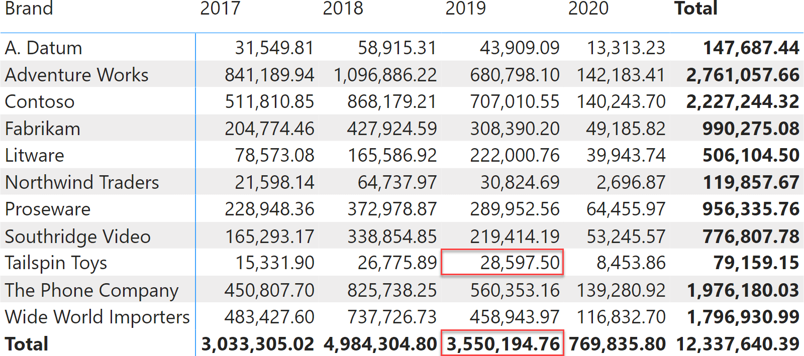
Despite containing subtotals and data well-organized in rows and columns, the matrix is generated from a query that returns a flat table. The flat table contains rows for the inner cells, as well as rows for the subtotals. Indeed, the base query (simplified) that retrieves data for the matrix is the following:
EVALUATE
SUMMARIZECOLUMNS (
    ROLLUPADDISSUBTOTAL ( 'Product'[Brand], "IsGrandTotalRowTotal" ),
    ROLLUPADDISSUBTOTAL ( 'Date'[Year], "IsGrandTotalColumnTotal" ),
    "Sales_Amount", 'Sales'[Sales Amount]
)
The output of this query contains the whole resultset. In the following excerpt, you can easily recognize the values for Tailspin Toys in 2019 and the column subtotal for the same year:
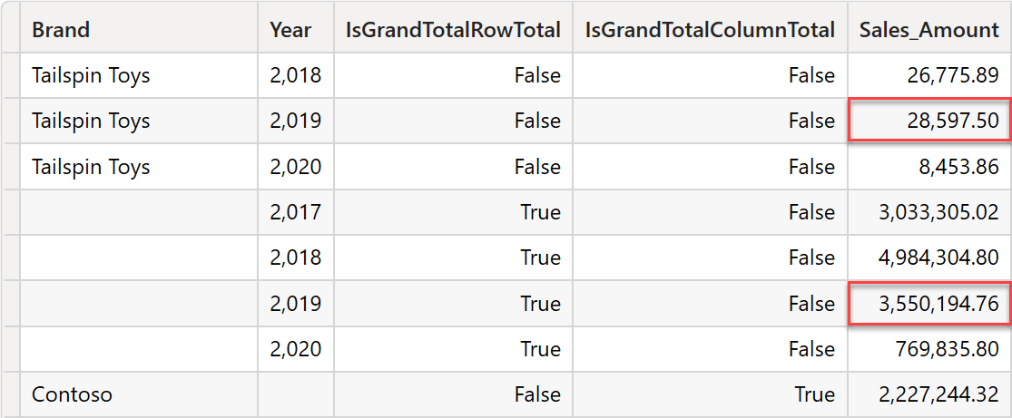
Power BI takes care of reading the flat table, detecting the subtotal rows (using the additional columns that indicate whether a row is a subtotal or not), and showing the values in the nice way we are used to reading a matrix.
It is important to recognize that the result of SUMMARIZECOLUMNS is flat: all the rows are at the same level, and there are no differences between a row containing a raw value and a subtotal. Power BI knows how to distinguish between subtotals and regular rows. From a DAX standpoint, however, all the rows are similar.
We can easily author a visual calculation that computes the growth, in percentage, between the previous value and the current value:
Growth =
VAR Curr = [Sales Amount]
VAR Prev = PREVIOUS ( [Sales Amount], COLUMNS )
VAR Result = DIVIDE ( Curr - Prev, Prev )
RETURN
    FORMAT ( Result, "0.00 %" )
The calculation uses the PREVIOUS function that returns the value of the previous column. Because the year is on the columns, PREVIOUS ( [Sales Amount], COLUMNS ) returns the previous year’s value. The calculation produces the following result.
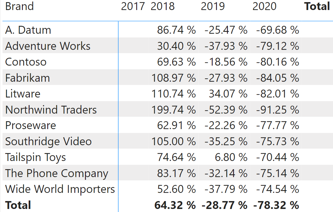
The Growth for 2017 is blank because there is no previous column, whereas the calculation produces a correct output in all the other years. The interesting question is: how does DAX know what the previous column is if the table returned by SUMMARIZECOLUMNS is just a flat table? The answer is in the VISUAL SHAPE clause added to the table returned by SUMMARIZECOLUMNS.
Let us take a look at a slightly simplified version of the query that produced the matrix above:
DEFINE
    COLUMN '__DS0VisualCalcs'[Growth] =
        (
            VAR Curr = [Sales Amount]
            VAR Prev =
                PREVIOUS ( [Sales Amount], COLUMNS )
            VAR Result =
                DIVIDE ( Curr - Prev, Prev )
            RETURN
                FORMAT ( Result, "0.00 %" )
        )
    VAR __DS0Core =
        SUMMARIZECOLUMNS (
            ROLLUPADDISSUBTOTAL ( 'Product'[Brand], "IsGrandTotalRowTotal" ),
            ROLLUPADDISSUBTOTAL ( 'Date'[Year], "IsGrandTotalColumnTotal" ),
            "Sales_Amount", 'Sales'[Sales Amount]
        )
    VAR __DS0VisualCalcsInput =
        SELECTCOLUMNS (
            KEEPFILTERS (
                SELECTCOLUMNS (
                    __DS0Core,
                    "Brand", 'Product'[Brand],
                    "IsGrandTotalRowTotal", [IsGrandTotalRowTotal],
                    "Year", 'Date'[Year],
                    "IsGrandTotalColumnTotal", [IsGrandTotalColumnTotal],
                    "Sales_Amount", [Sales_Amount]
                )
            ),
            "Brand", [Brand],
            "Year", [Year],
            "IsGrandTotalRowTotal", [IsGrandTotalRowTotal],
            "IsGrandTotalColumnTotal", [IsGrandTotalColumnTotal],
            "Sales Amount", [Sales_Amount]
        )
    TABLE '__DS0VisualCalcs' = __DS0VisualCalcsInput
        WITH VISUAL SHAPE
        AXIS ROWS
            GROUP [Brand]
                TOTAL [IsGrandTotalRowTotal]
            ORDER BY [Brand] ASC
        AXIS COLUMNS
            GROUP [Year]
                TOTAL [IsGrandTotalColumnTotal]
            ORDER BY [Year] ASC
        DENSIFY "IsDensifiedRow"
    VAR __DS0RemoveEmptyDensified =
        FILTER (
            KEEPFILTERS ( '__DS0VisualCalcs' ),
            OR (
                NOT ( '__DS0VisualCalcs'[IsDensifiedRow] ),
                NOT ( ISBLANK ( '__DS0VisualCalcs'[Growth] ) )
            )
        )
    VAR __DS0RemoveContextOnlyColumns =
        SELECTCOLUMNS (
            KEEPFILTERS ( __DS0RemoveEmptyDensified ),
            "'__DS0VisualCalcs'[Brand]", '__DS0VisualCalcs'[Brand],
            "'__DS0VisualCalcs'[Year]", '__DS0VisualCalcs'[Year],
            "'__DS0VisualCalcs'[IsGrandTotalRowTotal]",
                '__DS0VisualCalcs'[IsGrandTotalRowTotal],
            "'__DS0VisualCalcs'[IsGrandTotalColumnTotal]",
                '__DS0VisualCalcs'[IsGrandTotalColumnTotal],
            "'__DS0VisualCalcs'[Growth]", '__DS0VisualCalcs'[Growth],
            "'__DS0VisualCalcs'[IsDensifiedRow]", '__DS0VisualCalcs'[IsDensifiedRow]
        )
EVALUATE
    __DS0RemoveContextOnlyColumns
The query contains a lot of information to process:
- Visual calculations are created as query columns using DEFINE COLUMNS.
- The base query is the same as the previous matrix (see __Ds0Core).
- The base query undergoes several processing steps:
- Renaming of columns.
- Adding VISUAL SHAPE and the densification process.
- Removal of densified rows with no values in the visual calculations.
- Removal of columns used for the calculation but not required for the visual.
Each of these topics taken separately would be interesting and worth having its own article. In this article, we focus on the VISUAL SHAPE section.
The VISUAL SHAPE clause adds a hierarchical structure to an otherwise flat table:
    TABLE '__DS0VisualCalcs' = __DS0VisualCalcsInput
        WITH VISUAL SHAPE
        AXIS ROWS
            GROUP [Brand]
                TOTAL [IsGrandTotalRowTotal]
            ORDER BY [Brand] ASC
        AXIS COLUMNS
            GROUP [Year]
                TOTAL [IsGrandTotalColumnTotal]
            ORDER BY [Year] ASC
        DENSIFY "IsDensifiedRow"
The source of __DS0VisualCalcs is __DS0VisualCalcsInput, which is nothing but the original query after some of the columns have been renamed to match the local names. Indeed, visual calculations work by using the name of the column or measure in the matrix, rather than the name in the model. This is the reason for the renaming step. However, the original query does not contain the new columns added as visual calculations. On the other hand, __Ds0VisualCalcs contains the new columns.
VISUAL SHAPE defines one or two axes: ROWS, COLUMNS, or both. In the example, we have the definition of both ROWS and COLUMNS. For each axis, Power BI defines the grouping columns (Brand and Year, in the example), the name of the column that indicates whether a row is a subtotal or not, and their sort order. The last clause of VISUAL SHAPE is the name of the Densification column, a column added to the table to indicate whether the rows have been created because of densification.
In this first – simple – example, each axis has one level. However, when adding the Category and the Color on the rows, as well as the month on the columns, the result is more complex.
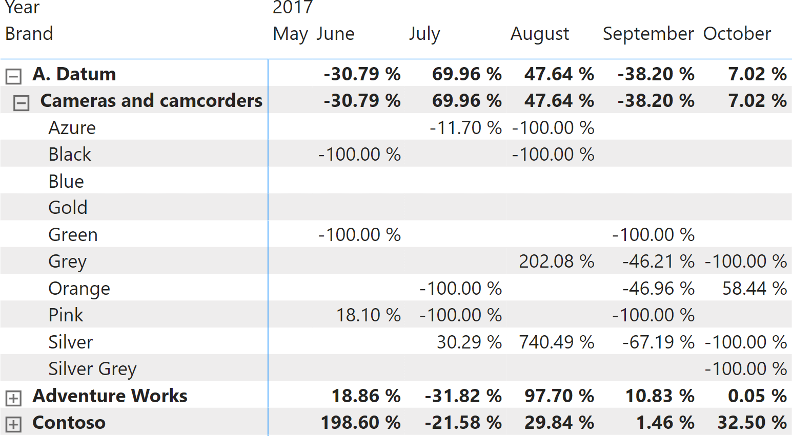
With a more complex hierarchical structure comes a more complex VISUAL SHAPE definition:
    TABLE '__DS0VisualCalcs' = __DS0VisualCalcsInput
        WITH VISUAL SHAPE
        AXIS ROWS
            GROUP [Brand]
                TOTAL [IsGrandTotalRowTotal]
            GROUP
                [Category],
                [Category_Code]
                TOTAL [IsDM1Total]
            GROUP [Color]
                TOTAL [IsDM3Total]
            ORDER BY
                [Brand] ASC,
                [Category_Code] ASC,
                [Category] ASC,
                [Color] ASC
        AXIS COLUMNS
            GROUP [Year]
                TOTAL [IsGrandTotalColumnTotal]
            GROUP
                [Month],
                [Month_Number]
                TOTAL [IsDM6Total]
            ORDER BY
                [Year] ASC,
                [Month_Number] ASC,
                [Month] ASC
        DENSIFY "IsDensifiedRow"
Each group of the axis contains the columns that define the hierarchy level and – if needed – the sort-by-column column, visible in both Category and Month levels.
The metadata added to the table by VISUAL SHAPE is the key for most visual calculation functions. Indeed, the code of Growth uses the keyword COLUMNS as the second argument of PREVIOUS:
Growth =
VAR Curr = [Sales Amount]
VAR Prev = PREVIOUS ( [Sales Amount], COLUMNS )
VAR Result = DIVIDE ( Curr - Prev, Prev )
RETURN
    FORMAT ( Result, "0.00 %" )
In this case, COLUMNS is a keyword that tells PREVIOUS to use the axis definition of COLUMNS to navigate the virtual table. Depending on the level at which the visual context is positioned, the engine knows it needs to navigate to the previous row of the virtual table using the sort order and the grouping defined in the axis.
ROWS and COLUMNS are keywords that can only be used in visual calculations. The reason is that the VISUAL SHAPE is created in the query made by Power BI. A regular model measure can access neither ROWS nor COLUMNS because a model measure can be added to a matrix that has no visual calculations in it. Therefore, it has no axis defined.
In conclusion, the first step that creates the environment in which visual calculations can be computed is the addition of metadata to the original result of SUMMARIZECOLUMNS through VISUAL SHAPE. It is worth noting that the table with VISUAL SHAPE is not a variable; it is a query-defined table. Because it is a table, the query can define new columns that are added to the table (columns cannot be added to variables). Each visual calculation is a new column added to the table, and these columns can reference ROWS and COLUMNS because the definition of the axis is part of the definition of the table.
Understanding the VISUAL SHAPE syntax is the first step in understanding how visual calculations are computed. Next, it is important to understand the lattice of levels defined by the axes and how EXPAND and COLLAPSE let developers navigate the lattice.
However, VISUAL SHAPE is already enough to figure out how functions like PREVIOUS and NEXT work. PREVIOUS and NEXT do not navigate the lattice. PREVIOUS is equivalent to OFFSET ( -1, ROWS ). The ability to reference ROWS lets users avoid the complexity of PARTITIONBY and ORDERBY, which are required to use OFFSET. ROWS is basically a shortcut to the group-by, the partition-by, and the order-by sections of a window function.
In this article, we just scratched the surface of the internals of visual calculations. We used some terms that require further description: the visual context, the current level, and the densification process. We will cover these topics in future articles. Our SQLBI+ readers interested in diving further into visual calculation will find the Visual Calculation whitepaper in their learning area in SQLBI+.
Evaluates an expression in a context modified by filters.
CALCULATE ( <Expression> [, <Filter> [, <Filter> [, … ] ] ] )
Retrieves a context with added levels of detail compared to the current context. If an expression is provided, returns its value in the new context, allowing for navigation in hierarchies and calculation at a more detailed level.
EXPAND ( [<Expression>] [, <Axis>] [, <Column> [, <Column> [, … ] ] ] [, <N>] )
Retrieves a context with removed detail levels compared to the current context. With an expression, returns its value in the new context, allowing navigation up hierarchies and calculation at a coarser level of detail.
COLLAPSE ( [<Expression>] [, <Axis>] [, <Column> [, <Column> [, … ] ] ] [, <N>] )
Create a summary table for the requested totals over set of groups.
SUMMARIZECOLUMNS ( [<GroupBy_ColumnName> [, [<FilterTable>] [, [<Name>] [, [<Expression>] [, <GroupBy_ColumnName> [, [<FilterTable>] [, [<Name>] [, [<Expression>] [, … ] ] ] ] ] ] ] ] ] )
The Previous function retrieves a value in the previous row of an axis in the Visual Calculation data grid.
PREVIOUS ( <Column> [, <Steps>] [, <Axis>] [, <OrderBy>] [, <Blanks>] [, <Reset>] )
The Next function retrieves a value in the next row of an axis in the Visual Calculation data grid.
NEXT ( <Column> [, <Steps>] [, <Axis>] [, <OrderBy>] [, <Blanks>] [, <Reset>] )
Retrieves a single row from a relation by moving a number of rows within the specified partition, sorted by the specified order or on the axis specified.
OFFSET ( <Delta> [, <Relation>] [, <OrderBy>] [, <Blanks>] [, <PartitionBy>] [, <MatchBy>] [, <Reset>] )
The columns used to determine how to partition the data. Can only be used within a Window function.
PARTITIONBY ( [<PartitionBy_ColumnName> [, <PartitionBy_ColumnName> [, … ] ] ] )
The expressions and order directions used to determine the sort order within each partition. Can only be used within a Window function.
ORDERBY ( [<OrderBy_Expression> [, [<OrderBy_Direction>] [, <OrderBy_Expression> [, [<OrderBy_Direction>] [, … ] ] ] ] ] )
Articles in the Visual Calculations series
- Introducing VISUAL SHAPE for visual calculations in Power BI
- Introducing EXPAND and COLLAPSE for visual calculations in Power BI
- Using EXPAND and COLLAPSE in visual calculations