Using EXPAND and COLLAPSE in visual calculations

In previous articles, we introduced the concepts of visual context, the visual lattice, and the two visual context navigation operations: EXPAND and COLLAPSE. In this article, we build on that knowledge to first compute a simple percentage over the parent: a simple calculation to consolidate the understanding of EXPAND and COLLAPSE. Next, we move on to a much more complex scenario, computing the inflation-adjusted sales using visual calculations.

Find more in the Understanding Visual Calculations in DAX whitepaper available to SQLBI+ subscribers

Computing the percentage over the parent

In the first example, we show how to compute the percentage over the parent. Creating the calculation is extremely easy because it is one of the predefined calculations of the visual calculations expression templates. However, our goal is not just to create the calculation, but rather, to understand how it works.

The calculation is % Parent, shown in the following figure.

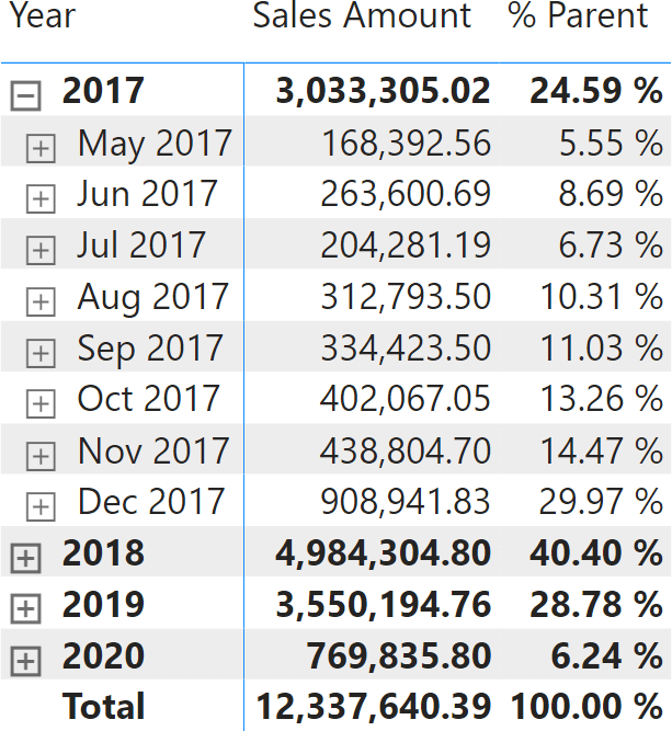
At each level of the hierarchy, the measure shows the percentage over the total of the parent level. Hence, May 2017 shows the ratio between 168,392.56 and 3,033,305.02. The code is rather simple:

% Parent = 
VAR Result = 
    DIVIDE ( 
        [Sales Amount],
        CALCULATE (
            [Sales Amount],
            COLLAPSE ( ROWS )
        )
    )
RETURN 
    FORMAT ( Result, "0.00 %" )

We included the FORMAT function in the code to show the values using the proper format string. Indeed, at the time of writing, it is not possible to define the format string of a visual calculation yet. The limitation is expected to be lifted before general availability; at that point, using a format string will be the preferred method of choosing the format of the measure.

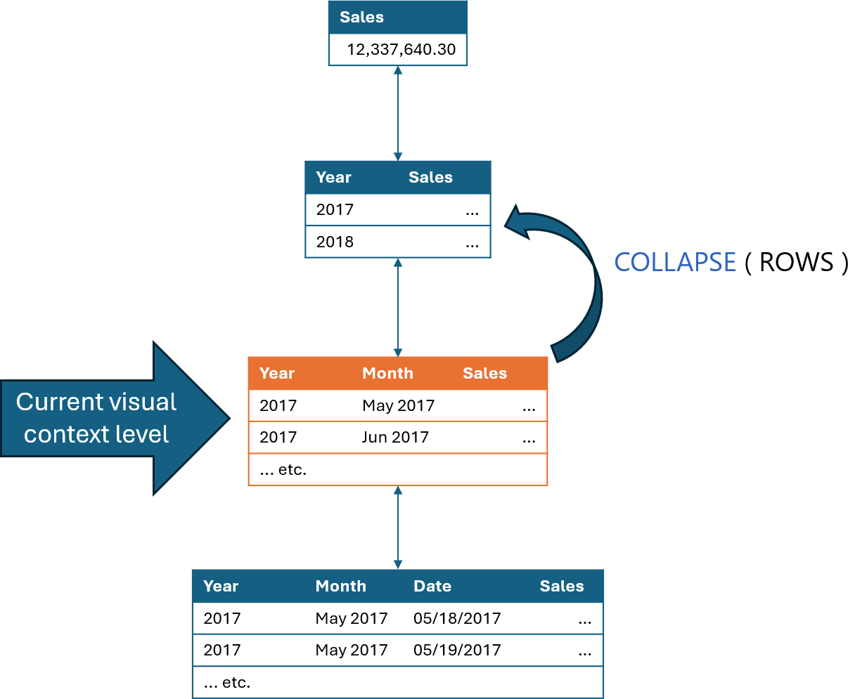
The key point in the visual calculation is using COLLAPSE as a navigation function in CALCULATE. COLLAPSE moves one step up from the level of the current visual context, navigating upwards in the visual lattice. When the visual context points to the Year-Month level, moving up produces the result at the Year level.

In the code, we used full syntax because we were interested in showing the nature of COLLAPSE as a CALCULATE navigation function. A shorter equivalent syntax would be the syntax-sugared version of COLLAPSE:

% Parent = 
VAR Result = 
    DIVIDE ( 
        [Sales Amount],
        COLLAPSE ( [Sales Amount], ROWS )
    )
RETURN 
    FORMAT ( Result, "0.00 %" )

It is worth remembering that the columns available in the virtual table depend on the level of the visual context. For example, the only columns available at the year level are Year and Sales Amount. The month column would evaluate to BLANK once you use COLLAPSE to move up one level.

This example was deliberately simple because we just wanted to refresh our knowledge about EXPAND and COLLAPSE. Let us now move on to the next example.

Adjusting sales based on inflation

Consider a scenario where a user wants to adjust the sales value based on inflation. The report needs to show both the sales amount and its value adjusted by applying the inflation rate up to the last day shown.

DAX offers many financial calculations, and maybe we can combine them to obtain the report. However, the nature of the article is educational. Therefore, we author the code from scratch to learn useful programming techniques.

Because the last month shown in the report is March 2020, the report applies inflation from 2017 to the end of March 2020 to the Sales Amount for 2017. It then repeats the same process for every following year considering the inflation until March 2020, which is the last month of data available. The granularity of the inflation is monthly. In other words, we want to apply the compound inflation rate, month-by-month, to all past sales.

Finally, we want to express the entire calculation with visual calculations. We also show the same calculation executed with a DAX measure to compare the two solutions at the end of the article.

The first problem is that we need a place to store the yearly inflation to compute the inflation adjustment. We could store the values on a model table. However, the very purpose of visual calculations is to allow users to create new calculations without having to change the model. Hence, a new visual calculation with a simple SWITCH seems very appropriate:

Yearly Adjustment = 
SWITCH (
    [Year-Month Year], 
    2017, 2.13,
    2018, 2.44,
    2019, 1.81,
    2020, 1.23
) / 100 + 1

-- Source: https://www.macrotrends.net/global-metrics/countries/USA/united-states/inflation-rate-cpi

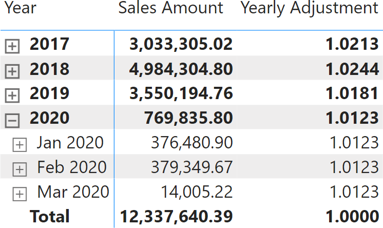
The next figure shows the visual calculation result, once properly formatted.

The next step is to compute the monthly adjustment. In the previous picture, you can see that the adjustment at the month level is the same as at the year level. We need to allocate the adjustment to the month level because our calculation needs to happen month by month. This requires us to compute the 12th root of the yearly adjustment to generate a number that—multiplied by itself 12 times—produces the correct value.

This monthly adjustment needs to be applied backwards. In other words, for February 2020, we need to apply the monthly adjustment of 2020 only once, and for January 2020, we need to apply the monthly adjustment of 2020 twice. 2019 is a bit more problematic because we have two different inflation rates: one for 2019 and one for 2020.

The algorithm needs to iterate over all the months after the current one and apply the monthly adjustment of the iterated year for each month. So the first variable we need to compute contains the months.

The months are contained in the virtual table, and we can access the virtual table through ROWS. ROWS, in a visual calculation, returns the set of rows at the current visual context level. However, we must compute the monthly granularity regardless of the current visual context level. For example, by computing ROWS when the visual context is at the year level, we obtain four rows, one per year. Doing the same at the individual date level would produce many more rows: one per day.

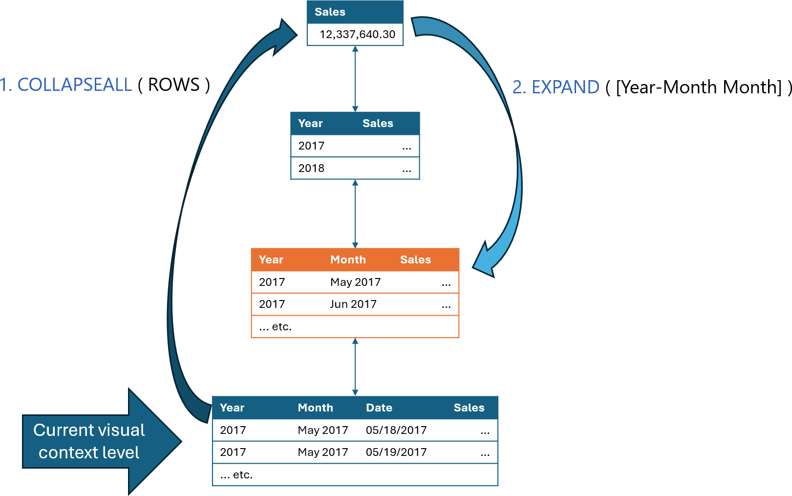
To make sure that ROWS is evaluated at the correct level for the visual context, we first go to the top of the hierarchy (with COLLAPSEALL), and we then use EXPAND to move to the month level:

VAR Months = 
    CALCULATETABLE (
        CALCULATETABLE (
            ROWS,
            EXPAND ( [Year-Month Month] )
        ),
        COLLAPSEALL ( ROWS )
    )

The following picture shows the two steps being executed: first, the outermost CALCULATETABLE executes COLLAPSEALL; then, the inner CALCULATETABLE executes EXPAND to move the visual context to the desired level.

The next step is to use a window function to obtain the list of all months after the current month and multiply the value of the monthly adjustment. In this case too, we need to ensure the calculation can be executed. Indeed, at the year level, there is no month. Therefore, we use EXPAND to move the visual context level to – at least – the month level:

VAR CumulativeAdjustment = 
    CALCULATE ( 
        PRODUCTX ( 
            WINDOW ( 1, ABS, -1, REL, Months, ORDERBY ( [Year_Month_Number], DESC ) ),
            POWER ( [Yearly Inflation], 1/12 )
        ),
        COLLAPSE ( [Year-Month Date] )
    )

Please note that to sort the Months variable properly, we needed to use an ORDERBY over the hidden Year_Month_Number column. Indeed, the column is part of the virtual table because it is needed for sorting. It is hidden, but it can be used freely.

The remaining part of the visual calculation is rather simple. Here is the full code:

Cumulative Adjustment = 
VAR Months = 
    CALCULATETABLE (
        CALCULATETABLE (
            ROWS,
            EXPAND ( [Year-Month Month] )
        ),
        COLLAPSEALL ( ROWS )
    )
VAR CumulativeAdjustment = 
    CALCULATE ( 
        PRODUCTX ( 
            WINDOW ( 1, ABS, -1, REL, Months, ORDERBY ( [Year_Month_Number], DESC ) ),
            POWER ( [Yearly Inflation], 1/12 )
        ),
        COLLAPSE ( [Year-Month Date] )
    )
VAR Result = 
    IF ( 
        ISATLEVEL ( [Year-Month Month] ), 
        COALESCE ( CumulativeAdjustment, 1 ) 
    )
RETURN
    Result

The Cumulative Adjustment column shows the multiplier to use – monthly – to adjust the Sales Amount value.

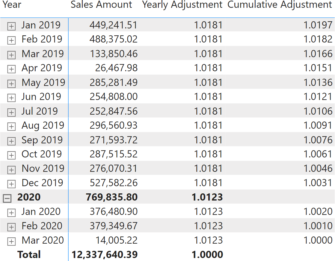
The final step is to multiply Sales Amount by Cumulative Adjustment. Please note that the Cumulative Adjustment column has no value at the year level. This is intentional, because the number cannot be computed at the year level: it must be computed month-by-month. The calculation below the month is fine because the daily sales will be multiplied by the monthly cumulative adjustment. At the year level, however, we must perform an iteration over the individual months.

Again, the calculation is simple, the key being the use of EXPAND to make sure that the iteration takes place at a visual level that includes the month:

Adjusted Sales = 
CALCULATE (
    SUMX (
        VALUES ( ROWS ),
        [Sales Amount] * [Cumulative Adjustment]
    ),
    EXPAND ( [Year-Month Month] )
)

EXPAND ensures that the calculation for the year and the grand total is moved down at the correct granularity. When at the month or day level, EXPAND does not move the visual context. Finally, note the use of VALUES ( ROWS ) rather than ROWS because of the different semantics of ROWS and COLUMNS in the visual context: ROWS is equivalent to ALL ( ROWS ); hence, VALUES (or DISTINCT) is required.

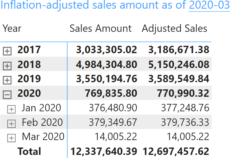
The next figure shows the result of Adjusted Sales.

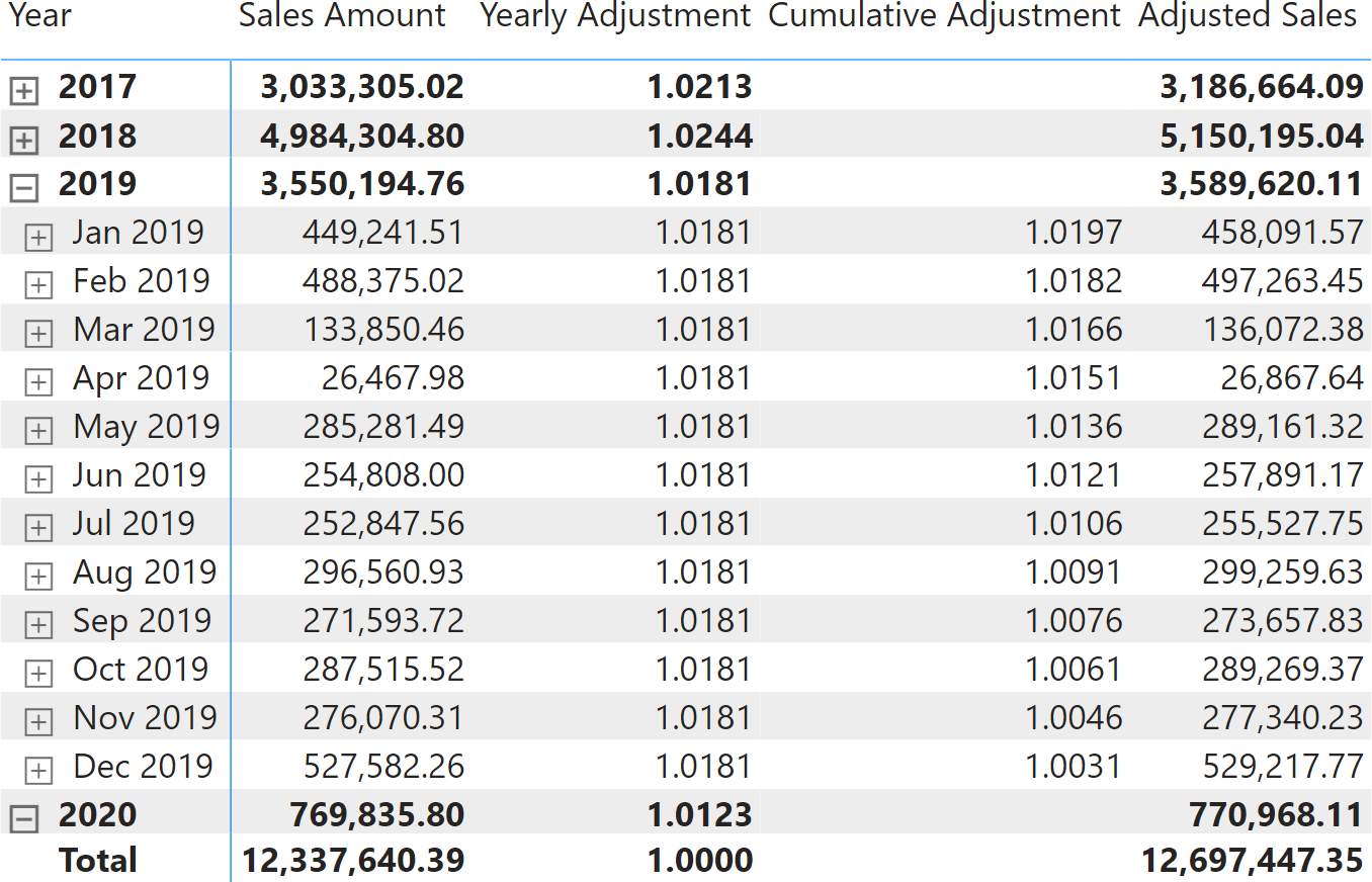
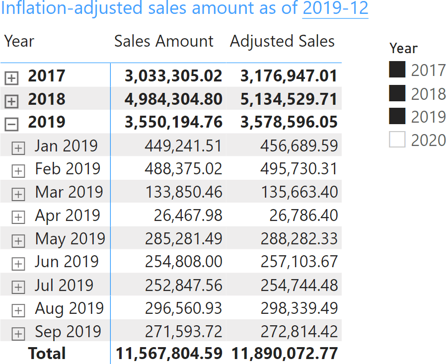
Hiding the columns that are not part of the report generates the desired result.

It is useful to note that the code also works in the presence of slicers filtering the visual. For example, filtering out 2020 produces different results for 2019 because the last row of the virtual table will be December 2019, leading to an inflation adjustment that references 2019 instead of 2020.

As you have seen, this second example is not trivial. Visual calculations leverage the full power of DAX and can perform complex calculations. However, as soon as the calculation complexity increases, it is necessary to move the visual context to the correct level to obtain the correct calculation.

It is interesting to examine the same calculation implemented through a regular DAX model measure. We used a similar approach for the algorithm, and this created a much longer version of the calculation:

VAR YearlyAdjustment =
    SELECTCOLUMNS (
        { ( 2017, 2.13 ), ( 2018, 2.44 ), ( 2019, 1.81 ), ( 2020, 1.23 ) },
        "Year", [Value1],
        "Yearly Adjustment", [Value2] / 100 + 1
    )
--
--  Find the last visible year-month for which there are sales,
--  so to define the date to use to compute the inflation
--
VAR LastVisibleYearMonth =
    CALCULATE (
        MAXX (
            SUMMARIZE ( Sales, 'Date'[Year Month Number] ),
            'Date'[Year Month Number]
        ),
        ALLSELECTED ()
    )
--
--  Convert the yearly inflation to the month level, removing periods
--  that are after the LastVisibleYearMonth and adding the Year Month Number
--  column, needed to join with Sales later
--
VAR MonthlyAdjustment =
    FILTER (
        SELECTCOLUMNS (
            GENERATE ( 
                YearlyAdjustment, 
                VAR CurrentYear = [Year]
                RETURN
                CALCULATETABLE (
                    VALUES ( 'Date'[Year Month Number] ),
                    REMOVEFILTERS ( 'Date' ),
                    'Date'[Year] = CurrentYear
                )
            ),
            "Year Month Number", 'Date'[Year Month Number],
            "Monthly Adjustment", POWER ( [Yearly Adjustment], 1 / 12 )
        ),
        [Year Month Number] <= LastVisibleYearMonth
    )
--
--  Compute, for each month, the cumulated inflation that we need to apply
--  to adjust the sales
--
VAR CumulativeAdjustment =
    ADDCOLUMNS (
        MonthlyAdjustment,
        "Cumulative Adjustment",
            VAR CurrentYearMonth = [Year Month Number]
            RETURN
                COALESCE (
                    PRODUCTX (
                        FILTER ( MonthlyAdjustment, [Year Month Number] > CurrentYearMonth ),
                        [Monthly Adjustment]
                    ),
                    1
                )
    )
--
--  Compute the sales by Year Month Number, so to join it later with 
--  the cumulative adjustment
--
VAR SalesByMonth =
    SELECTCOLUMNS (
        SUMMARIZE ( Sales, 'Date'[Year Month Number] ),
        "Monthly Sales", [Sales Amount],
        "Year Month Number", 'Date'[Year Month Number]
    )
--
--  Adjust sales by month, after a join with the cumulated inflation 
--
VAR SalesAdjusted =
    ADDCOLUMNS (
        NATURALLEFTOUTERJOIN ( SalesByMonth, CumulativeAdjustment ),
        "Adjusted Sales", [Monthly Sales] * [Cumulative Adjustment]
    )
VAR Result = SUMX ( SalesAdjusted, [Adjusted Sales] )
RETURN
    Result

The code is explained in the comments. It is worth noting that this time, there is no need to use a separate column to store the yearly adjustment. Indeed, we can use a variable and then allocate the monthly adjustment by accessing the model and creating the needed structures on the fly.

Moreover, it is necessary – in the measure – to compute the monthly sales amount and perform a NATURALLEFTOUTERJOIN with the cumulative adjustment. This operation is unnecessary in a visual calculation because the virtual table already contains the precomputed values.

Despite being more intricate, the model measure still presents several advantages:

It works even when the years and months are not part of the visual. If we were to compute the same report slicing by brand rather than by year and month, the model measure would still compute a correct result, whereas the visual calculation would not work.
It can be computed through a calculation group. Replacing [Sales Amount] with SELECTEDMEASURE would make the code suitable for a calculation item, enhancing its reusability.
It can be reused in any visual. The visual calculation—by its nature—lives in a visual and is tied to the visual structure. Despite being more complex to write, a model measure can be used anywhere (if well architected).

The DAX developer must choose which technique to use by carefully evaluating the pros and cons of each technique.

Conclusions

You can use visual calculations by just using the templates without having to worry about the complexity of the visual context, the level in the visual lattice, or how to navigate though it. However, using the templates as a starting point to learn exactly how visual calculations work is a nice step forward in your career as a DAX master. Once you learn the basics of visual calculations, you can enjoy more power and build more complex (and interesting) calculations.

However, visual calculations have several limitations. They can access only the virtual table, and they are strongly tied to the visual structure. Changing the visual structure may quickly invalidate your calculations, requiring major rewriting.

On the other hand, model measures are more complex to write, and they are less visual. However, a good DAX developer can create model calculations that are easier to use in any visual, driving the calculation by using tables and structures that are not visible in the matrix.

In other words, a good DAX developer needs to know both ways of computing values, and pick the right one for the specific scenario they are facing.

Find more in the Understanding Visual Calculations in DAX whitepaper available to SQLBI+ subscribers