Optimizing DAX with AI

NOTE: The solution in the video differs from the one in the article. We suggest comparing the article and video solutions to see how the same problem can yield different responses with the same context and prompts.

The debate over whether AI will replace human work is heating up. However, our vision is different: AI is not a replacement; it is a powerful tool, and when AI and humans work together on a problem, the outcome is better than when either works on their own.

Optimizing DAX is a fascinating task. However, in the process of optimizing DAX, you need to pay attention to several details:

The new formula needs to be equivalent to the old one; this requires extensive testing.
The shape of the query being executed matters: a formula may be better than another in a specific test, but not in others.
The data distribution matters: a database with 100K customers and 100M transactions requires a different optimization compared to one with 10K customers and 10B transactions.

The fascinating part is in finding new ways to express the same algorithm. All the details are quite boring, and it is easy to make mistakes because you need to run many tests. The good thing about AI is that it can generate and run tests for you, collect the results, and prepare reports that help you better understand whether a new formula is a good replacement for the old one. For this type of task, AI is a great assistant.

However, this article investigates a different question. Can AI optimize a DAX formula well? Optimizing requires specific skills: a certain knowledge of the DAX engine, the ability to generate different versions of the same algorithm, and a bit of creativity to test ideas that may look unorthodox but turn out to be smart in the complex world of columnar databases.

This article is not a complete paper about how effective AI can be at optimizing DAX. We tested a simple formula and drew some initial conclusions. Your mileage may vary, and things will change quickly as new LLMs emerge. However, in its simplicity, the article draws a simple idea:

AI can optimize DAX code, like a good developer. However, AI can produce better results when a human guides it toward new ideas. AI can further refine those ideas, and human-AI interaction can produce strong results.

When it is time to test AI, there is a subtle problem: if we ask it to optimize a formula we have already written, AI has seen it and is likely to find similar examples and adapt them to the new task. So, we needed an exotic calculation unlikely to appear online.

Here is an excerpt of the contract. You can find the full contract in the download content of this article.

Repeat purchase sales contract

Create a DAX measure named Repeat Purchase Sales. It returns sales made on purchase days that occur within 30 calendar days of the same customer’s immediately preceding purchase day.

Purchase days and qualification

Evaluate customers independently, using CustomerKey as their identity.

A purchase day is a distinct Order Date with at least one Sales row surviving the applicable business filters. Several order lines or orders on the same date form one purchase day. A second order on the same day does not establish a previous purchase day.

For each visible purchase day, find the immediately preceding, strictly earlier purchase day for that customer. That preceding day can be outside the visible date selection.

Include the current purchase day’s Sales Amount when the gap is between 1 and 30 calendar days, inclusive. Exclude the first purchase day in the available history and any day whose preceding purchase day is more than 30 days earlier. Include all selected sales lines on a qualifying day, exactly once.

Acceptance examples

With purchase days January 1, January 20, and February 25, January 20 qualifies, and February 25 does not. Selecting only January 20 must still find January 1.

A gap of exactly 30 days qualifies; a gap of 31 days does not.

If the only preceding purchase within 30 days is outside a selected category or store, it does not qualify the current day under that selection.

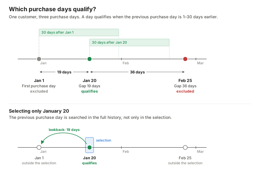
When asked to create the measure, AI generates this code:

Measure in Sales table

Repeat Purchase Sales =
SUMX (
    VALUES ( Customer[CustomerKey] ),
    VAR HistoricalPurchaseDates =
        CALCULATETABLE ( VALUES ( Sales[Order Date] ), REMOVEFILTERS ( 'Date' ) )
    VAR VisiblePurchaseDates =
        CALCULATETABLE ( VALUES ( Sales[Order Date] ) )
    RETURN
        SUMX (
            VisiblePurchaseDates,
            VAR PurchaseDate = Sales[Order Date]
            VAR PreviousPurchaseDate =
                MAXX (
                    FILTER ( HistoricalPurchaseDates, Sales[Order Date] < PurchaseDate ),
                    Sales[Order Date]
                )
            VAR GapDays = PurchaseDate - PreviousPurchaseDate
            RETURN
                IF (
                    NOT ISBLANK ( PreviousPurchaseDate ) && GapDays <= 30,
                    CALCULATE ( [Sales Amount] )
                )
        )
)

This measure works fine; it satisfies the contract. However, to a seasoned DAX developer, a few details immediately jump out:

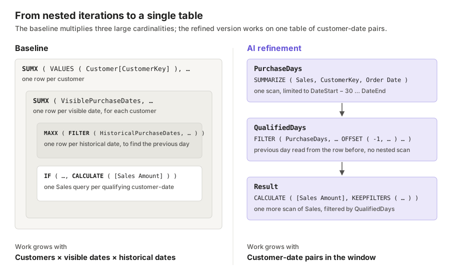
There are as many as three levels of nested iterations: an outer SUMX, an inner SUMX inside the RETURN part, and an even deeper MAXX over a FILTER. This is potentially bad.
The outer iteration has the cardinality of Customer; the inner iteration has the cardinality of Date. Both cardinalities are large. Also, the MAXX iteration has the cardinality of Date as well, which is not small. Multiplying those cardinalities produces a large number of rows to evaluate.
CALCULATETABLE inside SUMX (see VisiblePurchaseDates) can generate large temporary variables, thus producing inefficient code.

These are all signs of possible optimizations. The DAX engine will likely eliminate some iterations and replace them with table scans at a finer granularity; however, there is still room for improvement.

To challenge the AI, we first worked on the formula ourselves, creating our own optimized version:

Measure in Sales table

Repeat Purchase Sales (Human) =
VAR MaxDelta = 30
VAR DateStart = MIN ( 'Date'[Date] )
VAR DateEnd = MAX ( 'Date'[Date] )
VAR CustomersAndDates =
    ADDCOLUMNS (
        CALCULATETABLE (
            SUMMARIZE ( Sales, Customer[CustomerKey], Sales[Order Date] ),
            REMOVEFILTERS ( 'Date' ),
            'Sales'[Order Date] >= DateStart - MaxDelta && 'Sales'[Order Date] <= DateEnd
        ),
        "@SalesAmount", [Sales Amount]
    )
VAR AddDeltas =
    ADDCOLUMNS (
        CustomersAndDates,
        "@Delta",
            Sales[Order Date]
                - SELECTCOLUMNS (
                    OFFSET (
                        -1,
                        CustomersAndDates,
                        ORDERBY ( Sales[Order Date] ),
                        PARTITIONBY ( Customer[CustomerKey] )
                    ),
                    Sales[Order Date]
                )
    )
VAR Result = 
    SUMX ( 
        FILTER ( 
            AddDeltas, 
            [@Delta] <= MaxDelta && Sales[Order Date] >= DateStart 
        ), 
        [@SalesAmount] 
    )
RETURN
    Result

Here is the rationale behind the changes:

The formula first collects in CustomersAndDates the relevant pairs of customers and dates, along with the sales amount. The idea is to retrieve the sales amount during this scan to reduce the number of Sales scans. It looks promising, but it is not, as we will see later.
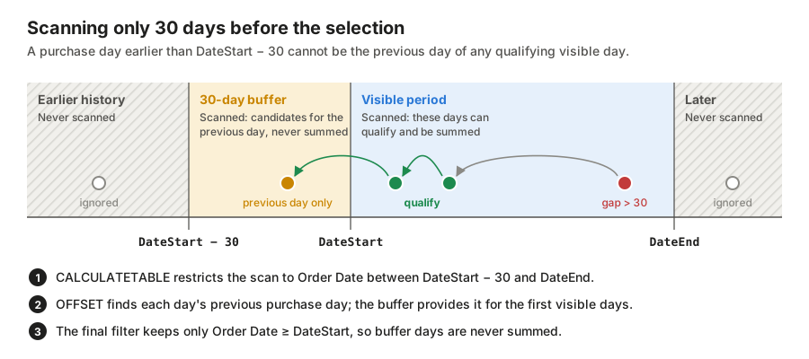
To reduce the size of the table, rather than scanning all dates, CustomersAndDates goes back no more than 30 days, because any transaction earlier than 30 days from the minimum is pointless for the algorithm.
We use the new OFFSET function to compute the previous order date, as OFFSET (being new) is more likely to be well-optimized.
The final FILTER is needed to avoid considering the additional earlier dates that are present in AddDelta, through CustomersAndDates.

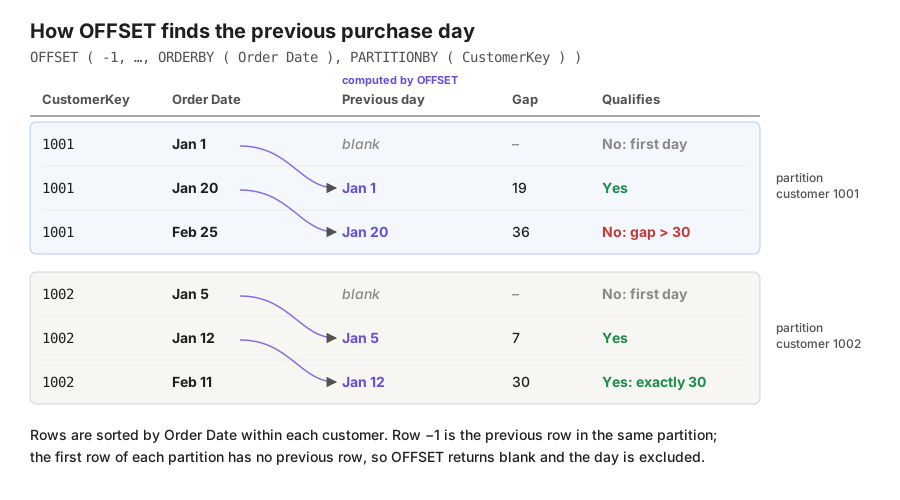
To produce this optimized version, we did not check the formula engine, storage engine, or other details. The formula structure makes it clear that the code is heavily dependent on the formula engine; therefore, the only good option is to reduce the size of the temporary tables.

At the same time, we asked AI to produce an optimized version of the original formula. Here is the result:

Measure in Sales table

Repeat Purchase Sales AI Independent = 
VAR FirstVisibleDate = MIN ( 'Date'[Date] )
VAR LastVisibleDate = MAX ( 'Date'[Date] )
RETURN
    SUMX (
        VALUES ( Customer[CustomerKey] ),
        VAR HistoricalPurchaseDates =
            CALCULATETABLE (
                VALUES ( Sales[Order Date] ),
                REMOVEFILTERS ( 'Date' ),
                'Date'[Date] >= FirstVisibleDate - 30,
                'Date'[Date] < LastVisibleDate
            )
        VAR VisiblePurchaseDays =
            CALCULATETABLE (
                SUMMARIZECOLUMNS ( Sales[Order Date], "@SalesAmount", [Sales Amount] )
            )
        VAR QualifyingPurchaseDays =
            FILTER (
                VisiblePurchaseDays,
                VAR PurchaseDate = Sales[Order Date]
                RETURN
                    COUNTROWS (
                        FILTER (
                            HistoricalPurchaseDates,
                            Sales[Order Date] < PurchaseDate 
                                && Sales[Order Date] >= PurchaseDate - 30
                        )
                    ) > 0
            )
        RETURN
            SUMX ( QualifyingPurchaseDays, [@SalesAmount] )
    )

There are some interesting details in the version created by AI:

It used the same optimization we found, limiting the temporary HistoricalPurchaseDates table to only 30 days earlier. This is honestly unexpected; we did not think AI could uncover this detail.
It uses SUMMARIZECOLUMNS inside an iteration to create VisiblePurchaseDays. We would not use SUMMARIZECOLUMNS inside a row context, even with a previous context transition, because it is scary, to say the least: the interactions between the logic of SUMMARIZECOLUMNS and the row/filter context are very complex to manage.
It precomputes Sales Amount inside SUMMARIZECOLUMNS, using a technique similar to what we did.
It still maintains multiple iterations. The outer iteration is SUMX over the customers, the inner iteration is FILTER over HistoricalPurchaseDates. However, it reduced the number of nested iterations.

During this optimization phase, the AI agent not only created a new version of the code but also generated an extensive set of queries to verify that the new measure is functionally equivalent to the old measure.

The query is too long to show here – again, see the download section. However, it is a gigantic set of subqueries like this:

    ROW (
        "Test", "01 First purchase day is blank",
        "Expected", BLANK (),
        "Baseline", CALCULATE ( 
            [Repeat Purchase Sales Baseline],
            TREATAS ( { 245745 }, Customer[CustomerKey] ),
            TREATAS ( { DATE ( 2016, 9, 7 ) }, 'Date'[Date] ) ),
        "Candidate", CALCULATE ( 
            [Repeat Purchase Sales Under Test],
            TREATAS ( { 245745 }, Customer[CustomerKey] ),
            TREATAS ( { DATE ( 2016, 9, 7 ) }, 'Date'[Date] ) )
    )

It runs the two measures under well-known test cases that verify edge-case scenarios, then checks that the results match.

Let us be very honest. We have optimized thousands of DAX measures in the last 15 years. We have never prepared such an extensive set of tests, even though we knew we should have. We just never had the time and the patience to build the test sets. The fact that AI does not get bored and is also very precise when writing code makes it worth integrating into the optimization process.

Next, it prepared a set of queries to test the performance of the measures. Again, it identified a few test scenarios:

One full year
Grouping by month in a full year
Grouping by month and country in a full year
Grouping by month and category in a full year
One large, big total with no grouping

The selection of the test set of performance queries is smart. It performs grouping by different columns in different tables, using time as the primary grouping column. It accurately checks how different granularities affect the measured metric. Very well done.

Here are the results – in milliseconds – of the three versions:

Test query	Baseline	Human version	Independent AI
10 — 2025 total	1,244	354	340
11 — By month	998	866	705
12 — Month × country	1,166	891	715
13 — Month × category	2,710	1,678	1,345
14 — All-history total	4,396	2,594	3,910

As you can see, there is no clear winner. The AI-generated version is better in some scenarios and worse in others. With different data distributions, the results would be different again. However, it is fair to say the AI-optimized version is not bad at all. This is not the place for a deep dive, but the biggest gain is the shift to 30-day earlier dates, which both optimizations achieve.

The story could end here, with a substantial draw between SQLBI and AI. However, as we said in the introduction, this was never a contest. This study aims to identify the best way to use AI in the optimization process. Therefore, we asked AI to further optimize our version. The result is a small change that makes all the difference:

Measure in Sales table

Repeat Purchase Sales AI =
VAR DateStart = MIN ( 'Date'[Date] )
VAR DateEnd = MAX ( 'Date'[Date] )
VAR PurchaseDays =
    CALCULATETABLE (
        SUMMARIZE ( Sales, Sales[CustomerKey], Sales[Order Date] ),
        REMOVEFILTERS ( 'Date' ),
        Sales[Order Date] >= DateStart - 30,
        Sales[Order Date] <= DateEnd
    )
VAR QualifiedDays =
    FILTER (
        PurchaseDays,
        VAR PurchaseDate = Sales[Order Date]
        VAR PreviousPurchaseDate =
            MAXX (
                OFFSET (
                    -1,
                    PurchaseDays,
                    ORDERBY ( Sales[Order Date], ASC ),
                    PARTITIONBY ( Sales[CustomerKey] )
                ),
                Sales[Order Date]
            )
        RETURN
            PurchaseDate >= DateStart
                && NOT ISBLANK ( PreviousPurchaseDate )
                && PurchaseDate - PreviousPurchaseDate <= 30
    )
RETURN
    CALCULATE (
        [Sales Amount],
        KEEPFILTERS ( QualifiedDays )
    )

As you can see, the AI agent did not compute the sales amount in the initial SUMMARIZE. Instead it scanned the Sales table again at the end, using the QualifiedDays variable as a filter in CALCULATE. The remaining part of the code is basically identical to mine.

The results, in milliseconds, are very interesting:

Test query	Baseline	Human version	AI refinement	Independent AI
10 — 2025 total	1,244	354	236	340
11 — By month	998	866	775	705
12 — Month × country	1,166	891	730	715
13 — Month × category	2,710	1,678	1,299	1,345
14 — All-history total	4,396	2,594	1,538	3,910

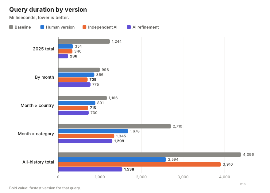
Overall, if this were a competition, our measure, further optimized by the agent, would win. Since this is not a competition, it just shows a lot about how to optimize code with AI.

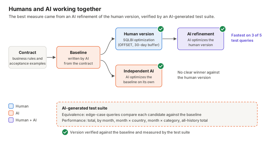
AI is not a replacement for humans. Its results are good, but not exceptional. The same goes for humans. If we had been left to work on this more deeply, we would probably have tested the AI-refined version and found a better one. However, AI found the best version much more quickly than we ever could. Moreover, an extensive set of queries supported the findings by validating that all tested measures use the same logic, and the tests used multiple, well-crafted queries that verified different query structures.

We are only scratching the surface of what AI-centered development can do; using AI in the optimization process is definitely valuable.