 Marco Russo
When you create a data model in Power BI, Power Pivot, or Analysis Services Tabular, every time you have two or more tables, you are likely to define relationships between them. These structures are important to simplify DAX queries, because of the automatic propagation of the filter context. They are also important for performance, because the storage engine queries are more efficient whenever the filter context propagates through relationships instead of by using DAX expressions (such as in the simulation of a relationship at different granularities described in Handling Different Granularities pattern). Nevertheless, there is a cost associated with relationships, which can have an impact in performance.
The relationship has to be relatively small, because it is a structure that the VertiPaq engine often reads executing queries. You can see its size in the Relationships page of the VertiPaq Analyzer, and you should start to concern when its size does not fit in CPU cache. In that case, the overhead of the RAM access might affect your query in a very negative way. It is hard to provide an absolute limit, because it depends on hardware, on other activities executed at the same time, and on the level of cache that can fit the structures used during the storage engine work. However, I will try to give some rule of thumb later in this article.
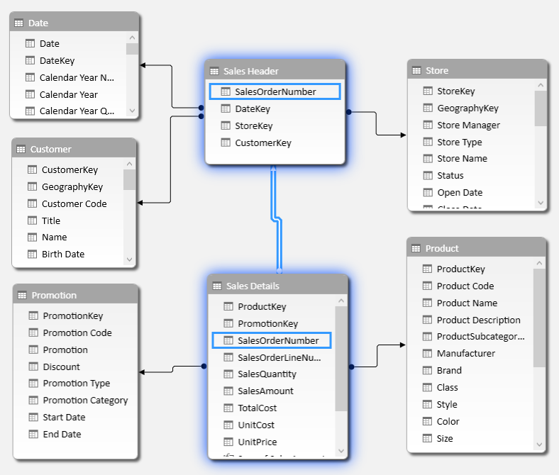
For example, consider the following structure. There are two tables, Sales Header and Sales Details, coming from typical Orders, Invoice, or Sales tables from an ERP. All the information related to the header are in one table, so that the table with the details of each line of the order/invoice contains does not duplicate these information, but only stores the identifier of the header row (SalesOrderNumber in this case).
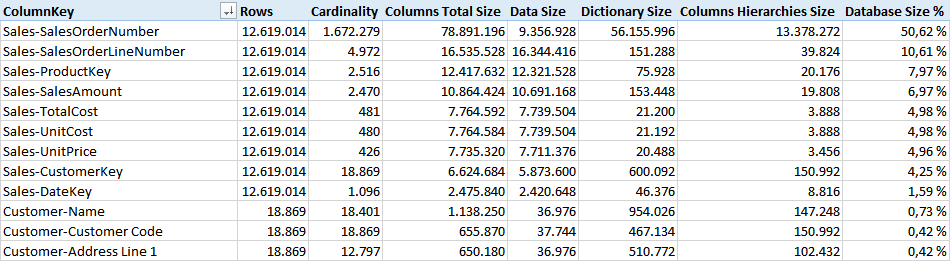
In the data model, the column we used to join Sales Header and Sales Details is the most expensive one, as you see from the Columns information provided by the VertiPaq Analyzer report. Such a column in the two tables require 91% of the memory of the entire model.
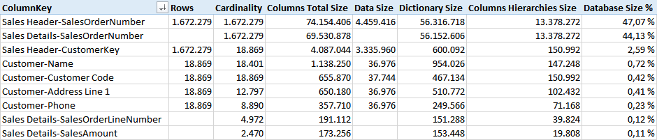
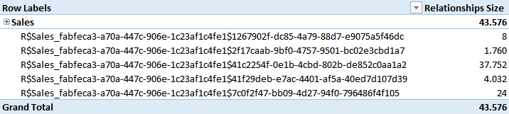
Dictionaries and hierarchies make the larger part of this cost, and a query that only uses the column to join the two tables will not use these structures. A more interesting number is the size of the relationship structure, available in the Relationships information provided by VertiPaq Analyzer.
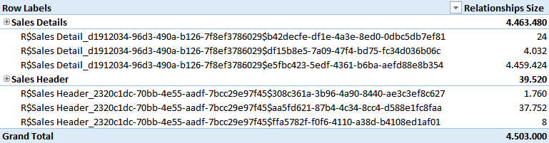
As you see, the Sales Details table has a relationship that requires more than 4 MB of memory. This number is directly related to the cardinality of the column involved in the relationship. In this case, it is already more than 4 MB, a number that might be already close if not over the limit of the available CPU cache.
For example, the following query requires 31 milliseconds to execute, and a storage engine CPU time of 141 milliseconds thanks to parallelism (time will vary on different hardware). As you see, there are no references to the SalesOrderNumber column, but the engine internally uses the relationship between Sales Header and Sales Details.
EVALUATE
ADDCOLUMNS(
    ALL ( Customer[Education] ),
    "Sales Amount", [Sum of SalesAmount]
)
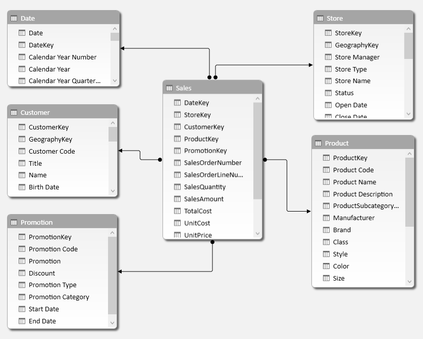
The alternative modeling approach is having a single denormalized table, Sales, which results from the join between Sales Header and Sales Details. The result you see in the following diagram is a regular star schema.
In this case, the cost of the columns is different and distributed across columns that were smaller in the normalized model. The difference is mainly in Data Size.
The relationships cost is now much smaller. All of them require less than 50 KB of memory.
Running the same simple query you have seen before requires now only 12 milliseconds, and a storage engine CPU time of 47 milliseconds (time will vary on different hardware). In a simple case like this one, the denormalization to a star schema saved 61% of the time. We run the test with 12 million rows in the Sales / Sales Details tables, but with a larger table and more complex DAX queries, the performance difference might increase, reaching easily one order of magnitude, and two order of magnitude if the size of the relationship increases over the size of all the CPU cache levels available.
As anticipated, there are a few rules of thumb to follow:
- Detect cardinality of columns involved in relationships
- Try to avoid relationships with lookup tables (on the one side of the relationship) having more than 5-10 millions of rows. Consider denormalization in the larger table (on the many side of the relationship), or move frequently queried columns with low-cardinality in a separate table with a smaller number of rows.
- Carefully monitor performance of relationships with lookup tables having between 200,000 and 5,000,000 of rows. You might apply the same optimization described before in case you detect performance degradation on specific hardware.
VertiPaq is an exceptional engine scanning large tables, also with billions of rows. However, it suffers more for the cardinality of the column used in a relationship. When you design a star schema, which is the suggested design pattern for this technology, this translates in a bottleneck when you have large dimensions, where large is something that has more than 1-2 million rows. Depending on the hardware, your yellow zone might range between 500,000 and 2,000,000 rows in a dimension. You definitely might expect performance issues with dimensions larger than 10,000,000 rows.
In The Definitive Guide to DAX you can learn how to find when this bottleneck is hit by a query reading information provided by SQL Server Profiler and DAX Studio, and how to optimize the data model in order to improve the efficiency of your query in similar conditions.