Understanding DAX Auto-Exist

Auto-exist is a technology built into DAX with the simple goal of avoiding useless calculations. In other words, it is an optimization technique used by the filtering mechanisms of DAX with the goal of reducing the effort of computing values.

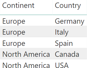
For example, imagine that one builds a report that slices by continent and country. In a database one might have two continents and five countries:

On this data, one might run a simple query like the following:

EVALUATE
SUMMARIZECOLUMNS ( 
    Geography[Continent],
    Geography[Country]
)

How is the engine going to solve the query? There are a couple of options:

• Retrieving all the possible values of Continent, all the possible values of Country and then generating the cartesian product of the two. In our example, it would return 10 rows.
• Retrieving the existing values of the Continent and Country pair, returning only the existing ones. In our example, it would return 5 rows.

The first option does not seem very smart. Because Italy is in Europe, there is no point in returning a non-existing row containing the pair >Italy, North America>. Therefore, DAX uses the second option and it does so by using a mechanism known as auto-exist.

The auto-exist mechanism kicks in when two or more columns of the same table are filtered together. Instead of using the columns as separate filters, SUMMARIZECOLUMNS generates only one filter which filters all the columns with only the existing combinations of values. Therefore, instead of scanning all the possible combinations (in our example this would mean 5 cities times 2 continents for a total of 10 combinations) the engine only scans the five existing combinations. Most of the times this is exactly what the user requested, only retrieved quicker as a table might have many more rows with duplicated values for the columns considered. Moreover, in the unlikely scenario where one wants to retrieve all the combinations, there are other table functions like CROSSJOIN that can generate non-existing combinations of values.

Nevertheless, there are scenarios where auto-exist might produce surprising results. Even seasoned DAX coders might fall into the trap of auto-exist, thinking that they are dealing with a bug when it is just auto-exist messing up the calculations.

In order to visualize the problem, we use a very small data model with just a few rows. The model contains one table with 9 rows:

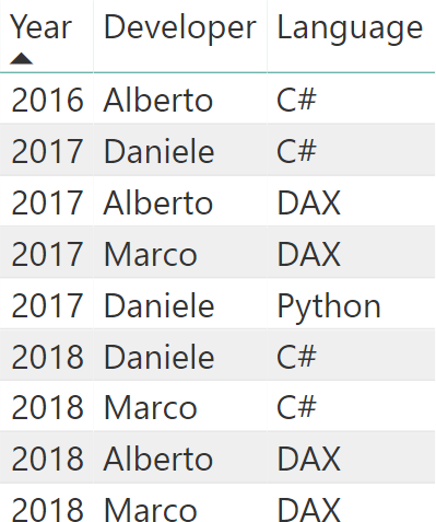
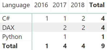
We have three developers that have developed projects in different languages over the years. Based on this table, a pivot table is useful to check how many languages were used in different years:

Then, we author a couple of simple measures:

# Projects = COUNTROWS ( Projects )

# Projects All Time = CALCULATE (
    [# Projects], 
    ALL ( Projects[Year] )
)

Finally, we use these measures in a dashboard that lets the user select year and language, and quickly see how many projects we covered in a selected year compared to the total number of projects over all time:

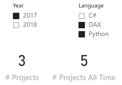
You can easily check the numbers against the previous matrix, or you can just trust our judgement: they are correct. The problem arises as soon as instead of selecting 2017, the user selects 2018:

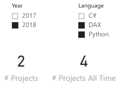
The number of projects is correct: two. However, the number of projects over all time has changed to an inaccurate value: four. It should still be five. How is this possible? This is not a bug. This is auto-exist messing up the calculation. Understanding how requires you to pay attention to a few details.

Once cleaned up, the query executed to retrieve # Projects All Time looks like the following:

EVALUATE
SUMMARIZECOLUMNS (
    TREATAS ( { "DAX", "Python" }, 'Projects'[Language] ),
    TREATAS ( { 2018 }, 'Projects'[Year] ),
    "Result", [# Projects All Time]
)

The two slicers generate two filters: one on the language, the other on the year. Pay attention to this detail: they are two slicers in Power BI, but when transformed in a query they are merged into a single call to SUMMARIZECOLUMNS.

Therefore, SUMMARIZECOLUMNS receives two filters on columns of the same table. This is when auto-exist kicks in. Being columns of the same table, they are merged together into a single filter that contains both columns and that only filters the existing values. Unfortunately, there is no row for Python in 2018. Therefore, the resulting filter only contains (2018, DAX).

When the measure starts, it removes the filters from the year by using ALL. Nevertheless, removing the filter on the year does not show Python. The filter context will only contain DAX, because Python has already been removed earlier by auto-exist. Another way of looking at it would be to say that the two filters received by SUMMARIZECOLUMNS are merged as if the query were expressed this way:

EVALUATE
SUMMARIZECOLUMNS (
    CALCULATETABLE (
        SUMMARIZE ( Projects, 'Projects'[Language], 'Projects'[Year] ),
        TREATAS ( { "DAX", "Python" }, 'Projects'[Language] ),
        TREATAS ( { 2018 }, 'Projects'[Year] )
    ),
    "Result", [# Projects All Time]
)

If you are curious, you can evaluate the CALCULATETABLE part on its own; you will see that Python is not part of the result.

Auto-exist is used only if multiple columns from the same table are used as filters. If the columns in the filters do not belong to the same table, then SUMMARIZECOLUMNS uses a cross-join operation instead of auto-exist. This obviously worsens performance. For example, instead of using a single table, we can build a regular star schema like in the following figure:

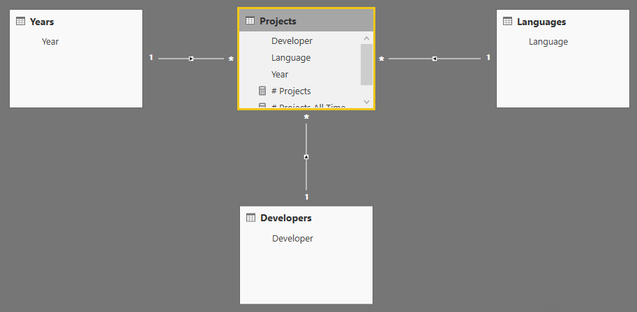
This small update completely changes the way SUMMARIZECOLUMNS works. First, we need to update the code of the measure:

# Projects All Time = CALCULATE (
    [# Projects], 
    ALL ( Years[Year] )
)

Then, instead of filtering by using the columns in the Projects table, we use the dimensions around the table. This transforms the query into the following:

EVALUATE
SUMMARIZECOLUMNS (
    TREATAS ( { "DAX", "Python" }, 'Languages'[Language] ),
    TREATAS ( { 2018 }, 'Years'[Year] ),
    "Result", [# Projects All Time]
)

Although the query looks the same as the previous one, you should notice that the filtering now happens on two tables: Languages and Years. Because the columns now belong to different tables, auto-exist does not kick in and the result is, as expected, five.

It is worth noting that auto-exist is executed by SUMMARIZECOLUMNS, and not by CALCULATETABLE. CALCULATETABLE does not perform auto-exist. Instead, it generates filters exactly as expected without the auto-exist step. The following query returns five, as desired.

EVALUATE
CALCULATETABLE (
    { [# Projects All Time] },
    TREATAS ( { "DAX", "Python" }, 'Projects'[Language] ),
    TREATAS ( { 2018 }, 'Projects'[Year] )
)

One might wonder why SUMMARIZECOLUMNS behaves this way. The reason is that SUMMARIZECOLUMNS is optimized for queries and auto-exist greatly reduces the space that the engine needs to scan to produce a result. In a regular star schema where dimensions are linked to the fact table, auto-exist only operates on dimensions. And because a model typically scans values from the fact table, it does not create any issues.

In simpler data models with only one table and with a fancy data distribution of values, it might be possible to run into auto-exist problems. When this happens, the easiest solution is to avoid using a single table and to build a proper star schema instead.

The golden rule of data modeling is always the same: always use star schemas. If a column has to be used to slice and dice, then it needs to belong to a dimension. Numbers to aggregate, on the other hand, are stored in fact tables. Tabular lets a developer deviate from the regular star schema architecture. This does not mean that doing it is always a good idea. It seldom is.