 Alberto Ferrari
Excel offers a simple function to compute the number of working days between two dates: NETWORKDAYS. DAX does not offer such a feature, so authoring more DAX code is required to compute the number of working days. The calculation can be written in several different ways, each one with pros and cons.
The purpose of this article is not to provide the best way to compute the number of working days. Instead, we want to show different versions of the same code, with an analysis of their complexity. This empowers developers to pick the appropriate approach according to the scenario they may be working with.
As our example, we consider the average delivery time of Contoso expressed in working days. As a reminder on working days, an order received on Friday and shipped on Monday has a delivery time of one day – Saturday and Sunday do not count.
Given a proper Date table with attributes set for day of week number, the easiest way to express this calculation is the following:
Average Delivery WD :=
AVERAGEX (                         -- Compute an average
    Sales,                         -- iterating over sales
    CALCULATE (                    -- Computing
        COUNTROWS ( 'Date' ),      -- the number of dates
        DATESBETWEEN (             -- that fall in between
            'Date'[Date],          --
            Sales[Order Date],     -- the order date
            Sales[Delivery Date]   -- and the delivery date
        ),                         -- Provided that they are not sat/sun
        NOT ( 'Date'[Day of Week Number] IN { 1, 7 } )
    )
)
This formula works fine. On the Contoso database with 12M rows in Sales, a simple query that computes the average delivery time per year runs very quickly. Nevertheless, in this article we are not interested in the execution time. We want to understand the complexity of the formula: what are the parameters affecting execution time?
The formula includes an outer iteration on Sales. It is thus likely to iterate 12M times, and each time it computes the filter arguments of CALCULATE. The first filter argument is DATESEBETWEEN, which returns the dates between Order Date and Delivery Date. The other filter is trivial and further investigation is not relevant.
The size of the table returned by DATESBETWEEN depends solely on the difference between Delivery Date and Order Date. The larger the difference, the larger the table returned by DATESBETWEEN.
In Contoso, all delivery times fall within a range of a few days. Therefore, the table is always very small leading to good performance. Nevertheless, there are many scenarios where events have a much larger duration and we wanted to test such scenarios. For the purpose of this demo we tweaked Contoso by adding 365 days to the Delivery date, just to add complexity and start our analysis.
This is the simple test query used:
EVALUATE
ADDCOLUMNS (
    VALUES ( 'Date'[Calendar Year] ),
    "WD", [Average Delivery WD]
)
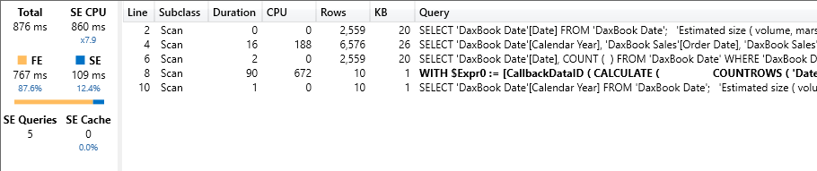
As expected, by increasing the delivery time, the execution time starts to grow: the test query now runs in 876 milliseconds, out of which 767 are formula engine (FE) time. Moreover, the query plan shows a nasty CallbackDataId, which is bad.
There are two factors that affect performance: the size of the fact table and the delivery time. We can work on both in order to improve performance.
There is no need to iterate over Sales to compute the average. Indeed, all the orders placed on one given day and delivered on another given day share the same delivery time. Therefore, one could reduce the iteration by taking all the distinct pairs of order date and delivery date. Before going any further, it is a good idea to evaluate whether it makes sense to try this out. How many distinct pairs of order and delivery date are there in Contoso? This simple query shows the result:
EVALUATE
{ (
    COUNTROWS ( Sales ),          -- Number of rows in Sales
    COUNTROWS (                   -- Compute the number of rows
        ALL (                     -- for all the distinct pairs
            Sales[Order Date],    -- of Order Date
            Sales[Delivery Date]  -- and Delivery Date
        )
    )

) }
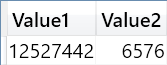
There are 12,527,442 rows in Sales, but only 6,576 distinct pairs of order date and delivery date. Thus, by reducing the top-level iteration we would expect a huge improvement in performance.
Time to roll up our sleeves and author a different version of the calculation. This time, it needs to iterate over the existing pairs of order date and delivery date, computing the number of orders that have the same pairs in the meantime. This is needed because the average will become a weighted average of the difference in working days, weighted by the number of rows:
Average Delivery WD :=
VAR NumOfAllOrders =
    COUNTROWS ( Sales )
VAR DeliveryWeightedByNumOfOrders =
    SUMX (
        SUMMARIZE ( Sales, Sales[Order Date], Sales[Delivery Date] ),
        VAR NumOfOrders =
            CALCULATE ( COUNTROWS ( Sales ) )
        VAR WorkingDays =
            CALCULATE (
                COUNTROWS ( 'Date' ),
                DATESBETWEEN ( 'Date'[Date], Sales[Order Date], Sales[Delivery Date] ),
                NOT ( 'Date'[Day of Week Number] IN { 1, 7 } )
            )
        RETURN
            NumOfOrders * WorkingDays
    )
RETURN
    DIVIDE ( DeliveryWeightedByNumOfOrders, NumOfAllOrders )
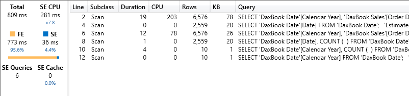
The code is no longer as simple as it was before. Moreover, when tested it is not even much faster than the previous code. It runs in 809 milliseconds, out of which 773 are FE time. The CallbackDataId is no longer present, but the huge amount of formula engine used is not a good sign.
Why was this optimization useless? Mainly because the DAX optimizer is pretty smart. In the first example, the iteration we required was an AVERAGEX over Sales. Nevertheless, the optimizer checked that the inner code of AVERAGEX did not depend on any column in Sales, apart from Order Date and Delivery Date. Thus, it already reduced the iteration to only the distinct pairs of Order Date and Delivery Date. This is not to say that reducing the cardinality of iterators is useless. In many scenarios the optimizer cannot understand the code well enough, in which case reducing iterator cardinality is usually a good choice. Here we were in a scenario where the optimizer was better than expected.
Time to work on the second part of the two optimizations available: if reducing the top-level iteration is not an option, we can reduce the size of the intermediate table returned by DATESBETWEEN. Indeed, instead of counting the number of working days between the two dates, we can count the number of non-working days. Typically, there are more working days than non-working days. Therefore, if we count the non-working days, the table will be smaller.
Following this idea, the next formula uses a different algorithm. It starts by computing a variable that contains the non-working days, then iterates over the distinct pairs of Order Date and Delivery Date, and for each pair it counts the non-working days filtering the variable computed previously.
Average Delivery WD :=
VAR NonWorkingDays =
    CALCULATETABLE (
        VALUES ( 'Date'[Date] ),
        ALL ( 'Date' ),
        'Date'[Day of Week Number] IN { 1, 7 }
    )
VAR TotalNumberOfSales =
    COUNTROWS ( Sales )
VAR DeliveryWeightedBySales =
    CALCULATE (
        SUMX (
            SUMMARIZE (
                Sales,
                Sales[Order Date],
                Sales[Delivery Date]
            ),
            VAR NumOfOrders =
                CALCULATE ( COUNTROWS ( Sales ) )
            VAR NonWorkingDaysInPeriod =
                COUNTROWS (
                    FILTER (
                        NonWorkingDays,
                        AND (
                            'Date'[Date] >= Sales[Order Date],
                            'Date'[Date] <= Sales[Delivery Date]
                        )
                    )
                )
            VAR DeliveryWorkingDays =
                Sales[Delivery Date]
                - Sales[Order Date]
                - NonWorkingDaysInPeriod
                + 1
            RETURN
                NumOfOrders * DeliveryWorkingDays
        )
    )
RETURN
    DeliveryWeightedBySales / TotalNumberOfSales
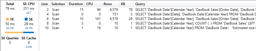
The algorithm is definitely not trivial, but it returns much better results than prior algorithms did.. Indeed, our query now runs in 79 milliseconds: around 10 times faster than the previous options. The amount of formula engine is still high: 50 milliseconds out of 79. Nevertheless, performance is now reasonable, at the cost of readability of course.
The biggest advantage of this formula is that it no longer depends on the duration of the event – it only depends on the number of non-working days in the period. This is not necessarily good news. In a model where the average duration is just a few days, this formula is not going to be the best performer. On the other hand, on a model where the average duration is several years, then it is likely to be your best option. As it always happens with DAX, there is no formula that works best in every scenario: we need to test and make educated decisions.
Finally, the best option to compute a complex value is not to compute it at all, or better to precompute it. Indeed, one could add a hidden calculated table to the model with the following code:
WD Delta =
ADDCOLUMNS (
    ALL (
        Sales[Order Date],
        Sales[Delivery Date]
    ),
    "Duration", [Average Delivery WD]
)
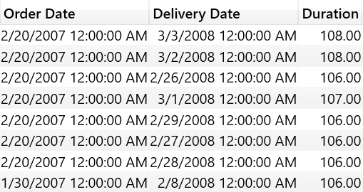
No matter how complex the code to compute the measure is, we are materializing in a table the number of working days between any two (existing) dates. At this point, the formula becomes much easier:
Average Delivery WD :=
VAR NumOfAllOrders =
    COUNTROWS ( Sales )
VAR DeliveryWeightedByNumOfOrders =
    SUMX (
        SUMMARIZE (
            Sales,
            Sales[Order Date],
            Sales[Delivery Date]
        ),
        VAR NumOfOrders =
            CALCULATE ( COUNTROWS ( Sales ) )
        VAR WorkingDays =
            LOOKUPVALUE (
                'WD Delta'[Duration],
                'WD Delta'[Order Date], Sales[Order Date],
                'WD Delta'[Delivery Date], Sales[Delivery Date]
            )
        RETURN
            NumOfOrders * WorkingDays
    )
RETURN
    DIVIDE (
        DeliveryWeightedByNumOfOrders,
        NumOfAllOrders
    )
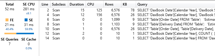
With the precomputed table, the whole calculation becomes a simple LOOKUPVALUE which searches for the precomputed value of the pair. This measure runs in 52 milliseconds, reducing complexity to a minimum.
This is not to say that one should precompute just any value in a model. Yet, precomputing values is always a good option. It is a very old technique that can still bring benefits even in the era of self-service BI.
Finally, some more optimization is possible in the formula engine by using NATURALLEFTOUTERJOIN instead of LOOKUPVALUE, as in this last version of the measure:
Average Delivery WD :=
VAR NumOfAllOrders =
    COUNTROWS ( Sales )
VAR SalesDates =
    SUMMARIZE ( Sales, Sales[Order Date], Sales[Delivery Date] )
VAR DatesDuration =
    TREATAS (
        SELECTCOLUMNS (
            'WD Delta',
            "Order Date", 'WD Delta'[Order Date],
            "Delivery Date", 'WD Delta'[Delivery Date],
            "Duration", 'WD Delta'[Duration]
        ),
        Sales[Order Date],
        Sales[Delivery Date],
        'WD Delta'[Duration]
    )
VAR DeliveryWeightedByNumOfOrders =
    SUMX (
        NATURALLEFTOUTERJOIN ( SalesDates, DatesDuration ),
        VAR NumOfOrders =
            CALCULATE ( COUNTROWS ( Sales ) )
        VAR WorkingDays = 'WD Delta'[Duration]
        RETURN
            NumOfOrders * WorkingDays
    )
RETURN
    DIVIDE ( DeliveryWeightedByNumOfOrders, NumOfAllOrders )
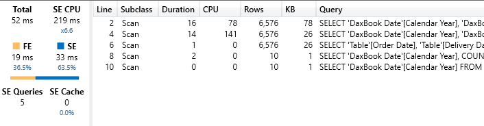
This version reduces the number of calls to LOOKUPVALUE, improving the performance if a single measure iterates over a large number of combinations of Order Date and Delivery Date. This measure runs in 52 milliseconds. There are no visible improvements compared to the previous version, but your mileage might vary on different datasets.
If you have enjoyed this article and want to better understand the internals of DAX to run your code faster, check out our Optimizing DAX video course: this is a focused, thorough series where we explain all the DAX optimization tools & tricks. .
Returns the number of whole workdays between two dates (inclusive) using parameters to indicate which and how many days are weekend days. Weekend days and any days that are specified as holidays are not considered as workdays.
NETWORKDAYS ( <start_date>, <end_date> [, <weekend>] [, <holidays>] )
Evaluates an expression in a context modified by filters.
CALCULATE ( <Expression> [, <Filter> [, <Filter> [, … ] ] ] )
Returns the dates between two given dates.
DATESBETWEEN ( <Dates>, <StartDate>, <EndDate> )
Calculates the average (arithmetic mean) of a set of expressions evaluated over a table.
AVERAGEX ( <Table>, <Expression> )
Retrieves a value from a table.
LOOKUPVALUE ( <Result_ColumnName>, <Search_ColumnName>, <Search_Value> [, <Search_ColumnName>, <Search_Value> [, … ] ] [, <Alternate_Result>] )
Joins the Left table with right table using the Left Outer Join semantics.
NATURALLEFTOUTERJOIN ( <LeftTable>, <RightTable> )