Understanding the “can’t determine relationship between the fields” error in Power BI

When you create a Power BI matrix, you drag and drop columns in the matrix, then add some measures, and Power BI figures out on its own which combinations of values to show. The process is so intuitive that we mostly ignore the details. However, Power BI sometimes cannot figure out how to populate the matrix, thus producing the error: “can’t determine relationship between the fields”. Adding a measure fixes the problem, but why? In some other scenarios, Power BI shows many empty rows, eliminating many of them only when you add a measure. Power BI shows a subset of the values in other scenarios, even when no measure is involved.

The behavior results from a mix of features: some are DAX features, while others are Power BI features. Power BI creates the query in a special way if no measure is involved, using a bridge table to link the tables used in the matrix. DAX implements auto-exists and non-empty in SUMMARIZECOLUMNS. Let us dive a bit deeper by first understanding DAX features.

Introducing the execution of SUMMARIZECOLUMNS

Power BI uses SUMMARIZECOLUMNS as the primary querying function. Nearly all the visuals use SUMMARIZECOLUMNS to retrieve the values to show. For example, the following is a simple matrix showing Product[Category], Product[Subcategory], and the Sales Amount measure.

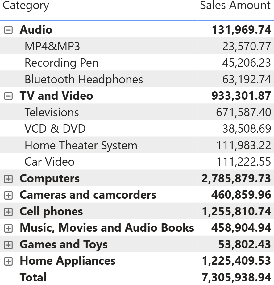
You can see that not all the combinations of category and subcategory are shown. For example, the Audio/Televisions combination is not in the list. The following query populates the matrix:

SUMMARIZECOLUMNS is used to group by four columns (categories are sorted by category code, and subcategories by subcategory code; hence, all four columns need to be present in the group-by list) and to compute the Sales Amount value.

SUMMARIZECOLUMNS produces the list of all the existing combinations of the four columns. Because all the columns come from the same table, SUMMARIZECOLUMNS is like a SUMMARIZE that groups the Product table by the four columns, computes the measure, and then removes rows that produce empty results. In other words, the code is equivalent to the following:

The SUMMARIZE part is known as “auto-exists”. SUMMARIZE generates only the existing combinations of values. This reduces the number of rows to evaluate, focusing on only the ones that make sense. The FILTER part is known as “non-empty”. SUMMARIZE removes the combinations that produce an empty result from the output. It is worth noting that SUMMARIZE uses Product, not Sales, as the starting table for grouping. For now, make a mental note about this small fact; it will be helpful later.

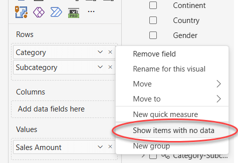
As we said, not all the combinations of category and subcategory are present in the matrix. A combination of values may be missing because of either auto-exists or non-empty operations. The net result is the same: the combination is not present. However, combinations removed by non-empty can be made visible, whereas combinations removed by auto-exists are never visible. In Power BI, you can use the “Show items with no data” option, to show combinations hidden by non-empty.

For example, let us add a slicer to only filter one city. This reduces the number of visible combinations.

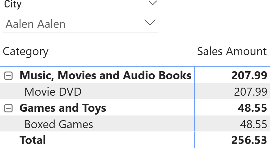
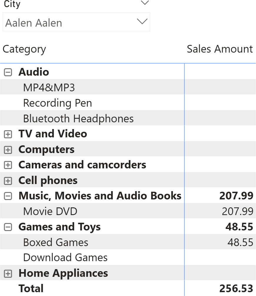
Forcing Power BI to show items with no data makes all the categories visible, and for each category, its subcategories. However, it does not show invalid combinations of category and subcategory.

Because of auto-exist, columns from the same table are grouped using SUMMARIZE. What happens when you add columns from different tables? In that scenario, SUMMARIZE is no longer an option; the tables are combined with CROSSJOIN.

In the following matrix, we added Store[Country] and Store[State] to the columns, keeping the filter for one city only. As you can see, there are only two stores that sell items to customers living in Aalen Aalen.

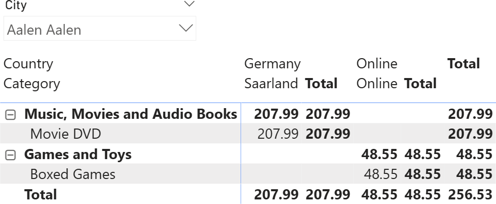
Because two tables are involved in the query, the two tables are summarized separately, and their result is cross-joined. This operation corresponds to the following query:

The important detail about the last query is that the summarized table is not, as one may expect, Sales. The two tables involved in the query (Store and Product) are summarized separately and later cross-joined. The resulting space is very large, including many combinations of columns from Store and Product that do not produce any value for the Sales Amount measure. Later, non-empty removes those empty rows that are still evaluated.

This is clearly visible by changing the definition of Sales Amount, where we add zero to avoid blanks:

This small change transforms the matrix into a monster with many rows and columns, all showing zero.

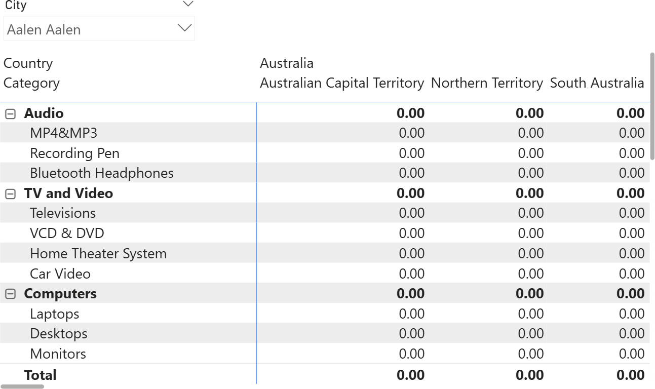
A similar behavior can be obtained by using the “Show items with no data” feature.

Hence, we have learned the most important details about SUMMARIZECOLUMNS: columns from the same table are summarized, their results are cross-joined, and non-empty removes the empty rows. Because non-empty removes most of the combinations, the measure being used in the matrix is the driver that defines what is shown in the matrix itself. If all the measures are evaluated as blank throughout an entire row, the row is removed from the output.

Understanding the error

Hence, the measures being used in a matrix define which rows to make visible. If no measure is being used, then SUMMARIZECOLUMNS produces the full cross-join. However, quite surprisingly, if we remove the Sales Amount measure from the matrix, we get the following result.

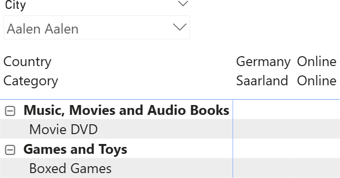
Despite no value being shown, only some of the combinations are visible. Namely, the same set of values shown previously when Sales Amount was present.

This behavior does not depend on DAX. Power BI detected that no measure is being computed for a given combination of model columns, and it tries to avoid showing the full cross-join by changing the query. Power BI (not DAX) determined that the two tables being used in the matrix are both related to Sales. Therefore, it generates a query that includes a measure that counts the rows in Sales to rely on the SUMMARIZECOLUMNS non-empty feature to reduce the rows being returned.

This is a simplified version of the query being executed:

As you see, it is Power BI that instructs SUMMARIZECOLUMNS to use Sales as a bridge table to reduce the number of rows. If no such table exists – that is, a table that can be filtered by the tables being used in the matrix and that acts as a natural bridge – Power BI produces an error.

We can easily check this by creating a copy of Store in a new calculated table (Unrelated Store):

Using columns from Unrelated Store rather than from Store produces an error in the matrix.

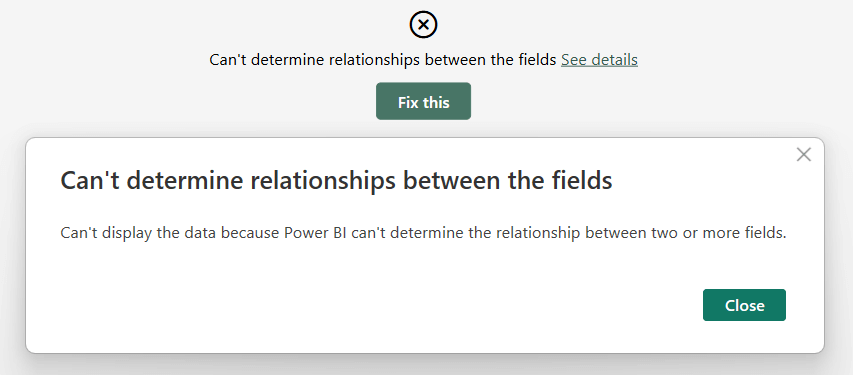
Adding any measure to the matrix removes the error, because – if a measure is present – then Power BI does rely on DAX to determine the values to show, rather than using its own algorithm – that is, searching for a suitable bridge table.

Conclusions

When you use a measure in a matrix, the measure itself is responsible for determining which rows to show. Two mechanisms are at work: non-empty and auto-exists. Auto-exists shows only the valid combinations of values from columns in the same table. Non-empty removes the rows in which all the measures evaluate to blank, from the output of SUMMARIZECOLUMNS.

If no measure were present, SUMMARIZECOLUMNS would produce a large result because it would cross-join all the summarized tables. Power BI prevents this large dataset from being returned by using a bridge table to reduce the number of rows shown.

Power BI produces an error if no bridge table can be found. Fixing this is easy: just add a measure to control which combinations you want to show.