 Alberto Ferrari
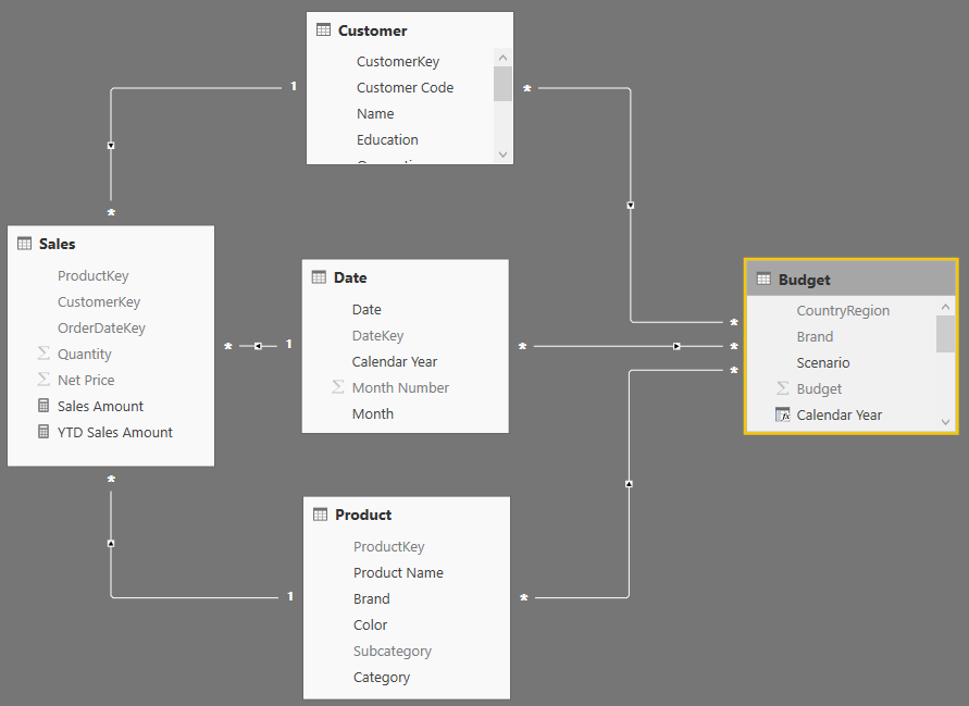
The data model used for this example contains two tables: Sales and Budget. The two tables are linked to Customer, Date, and Product through a set of relationships. They are strong relationships for the Sales table, which contains information at the key granularity; and weak relationships for the Budget table, which must be linked to the three dimensions at a different granularity.
Weak relationships are a new feature in Power BI. We will cover them in detail in a future article. We use the Budget table of the model to create several forecast measures. Here our main focus is on being able to prepare a chart like the following one:
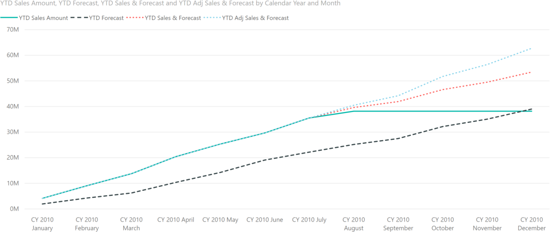
On the same chart the four lines represent these values:
- Green solid line: YTD Sales Amount is the year-to-date value of the actual sales. Because we only have sales until August 15, starting from August the line becomes flat.
- Black dashed line: YTD Forecast is the year-to-date of the budget. The chart shows that the budget predictions were too low, as Sales Amount is always much higher than Forecast.
- Red dotted line: YTD Sales & Forecast mixes the two values, using actual sales before August 15, and budget information after that date. The difference between this line and YTD Sales Amount starts to show at the end of August, because 15 days in August are already using budget values instead of actuals.
- Cyan dotted line: YTD Adj Sales & Forecast shows the actuals before August 15 and an adjusted value for the forecast. The adjusted forecast applies a correction to the budget based on the difference between budget and actuals in the previous months.
In order to understand the results of these measures, the following matrix shows the different values without the YTD calculation needed in the chart:
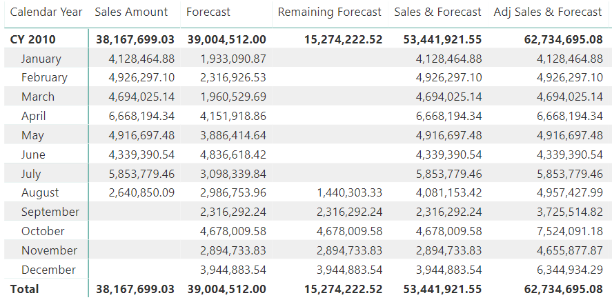
The Forecast measure in the demo model is quite an advanced piece of DAX code that would require a full article by itself. The curious reader will find more information on how to reallocate budget at different granularities in the video Budgeting with Power BI. In this article, we use the Forecast measure without detailed explanations; our goal is to explain how to compute the next measure: Remaining Forecast.
The Remaining Forecast measure must analyze the Sales table, finding the last day for which there are sales, and only then computing the forecasts. Here is the code:
Remaining Forecast :=
VAR LastDateWithSales =
    CALCULATE (
        MAX ( Sales[OrderDateKey] ),
        ALL ( Sales )
    )
VAR Result =
    CALCULATE (
        [Forecast],
        KEEPFILTERS ( 'Date'[DateKey] > LastDateWithSales )
    )
RETURN
    Result
There are just a couple of interesting notes about this formula: we had to use ALL on Sales when computing the LastDateWithSales variable to retrieve the last ever date with sales. Without the ALL modifier, the variable would compute the last date with sales in the filtered period (or context). This would return incorrect figures.
The other note is about the use of KEEPFILTERS when filtering the date in the Result variable. Because the filter operates on the DateKey column, which is the primary key of a table marked as a date table, it would override any previously existing filter. Therefore, KEEPFILTERS is needed in order to force the calculation within the currently selected time period.
You can appreciate the way the measure works, in August 2010. Because the last date with sales is August 15, in August the Remaining Forecast measure generates the forecast from August 16th until the end of the month.
The value of Remaining Forecast is then used by the Sales & Forecast measure, which simply sums the two base measures:
Sales & Forecast :=
    [Sales Amount] + [Remaining Forecast]
Bear in mind that the two measures can be summed easily, without the need for any extra tests. Indeed, Remaining Forecast only produces the value for future dates – at the same time, Sales Amount does not produce any value in future dates. Therefore, on any given day there are either sales or budget; both are never present at the same time.
Now, the second step: correcting the budget with the previous sales. As we already noted, the budget figures are too low. Applying a correction factor is a business requirement that should be addressed with much care. In this example we use a rather simple method: we compute the percentage difference between budget and sales up to August 15, and then we use this percentage difference as a correction factor for the future.
Here is the measure computing the percentage difference between budget and sales:
Yearly Delta % :=
VAR LastDateWithSales =
    CALCULATE (
        MAX ( Sales[OrderDateKey] ),
        ALL ( Sales )
    )
VAR Actual =
    CALCULATE (
        [Sales Amount],
        ALL ( 'Date' ),
        VALUES ( 'Date'[Calendar Year] )
    )
VAR BudgetComparison=
    CALCULATE (
        [Forecast],
        'Date'[DateKey] <= LastDateWithSales,
        VALUES ( 'Date'[Calendar Year] )
    )
VAR Result =
    DIVIDE (
        Actual - BudgetComparison,
        BudgetComparison
    )
RETURN
    Result
The measure is simpler than the previous one. It first computes the last date with sales (LastDateWithSales), then computes all sales in the current year (Actual) and the budget up to the last date with sales (BudgetComparison). The last division only transforms the difference into a percentage, which will be used later to update the budget figures.
The last step is using this percentage in the Adj Sales & Forecast measure, which computes the sales up to August 15 along with an adjusted version of the remaining forecast, corrected with the percentage:
Adj Sales & Forecast =
    [Sales Amount] + [Remaining Forecast] * ( 1 + [Yearly Delta %] )
In order to use these measures for the chart shown above, it is enough to embed them in a YTD pattern:
YTD Forecast :=
CALCULATE (
    [Forecast],
    DATESYTD ( 'Date'[Date] )
)

YTD Sales & Forecast :=
CALCULATE (
    [Sales & Forecast],
    DATESYTD ( 'Date'[Date] )
)

YTD Adj Sales & Forecast :=
CALCULATE (
    [Adj Sales & Forecast],
    DATESYTD ( 'Date'[Date] )
)
As you have seen, the code to author is not complex and the result is pretty nice. These measures are just the starting point of a complete budgeting solution. Nevertheless, they already show how you can produce powerful results in DAX, once you start mastering filter contexts and CALCULATE.
Returns all the rows in a table, or all the values in a column, ignoring any filters that might have been applied.
ALL ( [<TableNameOrColumnName>] [, <ColumnName> [, <ColumnName> [, … ] ] ] )
Changes the CALCULATE and CALCULATETABLE function filtering semantics.
KEEPFILTERS ( <Expression> )
Evaluates an expression in a context modified by filters.
CALCULATE ( <Expression> [, <Filter> [, <Filter> [, … ] ] ] )