UPDATE 2018-08-15: An additional technique to propagate a virtual relationship is available with TREATAS, described in the article Propagate filters using TREATAS in DAX.
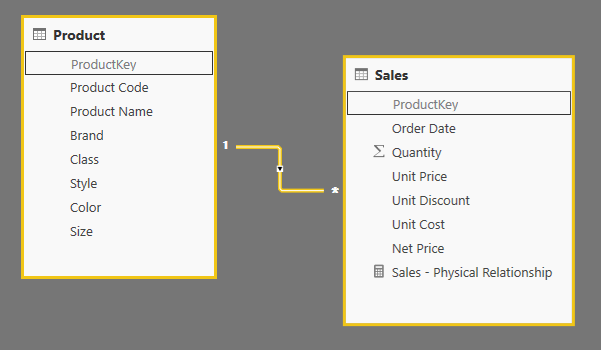
The more efficient way to apply a relationship between two tables is a physical relationship in the data model. For example, you can have a relationship between Sales and Product using the ProductKey column, as in the following schema.

In order to create a relationship in a data model in Power Pivot, Power BI, or Analysis Services Tabular, at least one side of the relationship must be tied to a column that is unique in the table. In this case, we connect the ProductKey column of the Product table (which is also the primary key) to the ProductKey column of the Sales table. This is the classical one-to-many relationship or a relational model.
Using this relationship, any filter over columns of the Product table is reflected in a filter of the Sales table. In other words, the relationship transfers the list of values filtered in the ProductKey column of the Product table, to a correspondent filter applied to the ProductKey column of the Sales table. This is done in a very efficient way at the storage engine level, and result in the best possible performance. You define a Sales Amount measure in a simple way, such as in the following definition.
[Sales - Physical Relationship] :=
SUMX ( Sales, Sales[Net Price] * Sales[Quantity] )
However, you might have scenarios where you do not have a physical relationship. The reason could be that tables have been imported without a relationship, and you cannot change the data model (for example, because you already deployed the data model in Analysis Services Tabular). However, a more common case is that you cannot create the relationship because none of the tables involved in the relationship has a column that satisfy the uniqueness condition required by a one-to-many relationship. You can find examples in the Handling Different Granularities pattern, but even tables that have multiple blank values in a column that would be unique otherwise has the same limit.
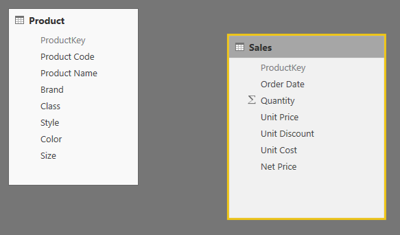
We can keep the example very simple, by just removing the relationship from our previous data model.
You can still obtain a valid measure by transferring the filter between the Product table and the Sales table using a specific filter argument in the CALCULATE function. For example, in any version of the DAX language (since Excel 2010), you can use the following technique (also described in the pattern we mentioned before).
[Sales - Virtual Relationship - 2012] :=
CALCULATE (
    SUMX ( Sales, Sales[Net Price] * Sales[Quantity] ),
    FILTER (
        ALL ( Sales[ProductKey] ),
        CONTAINS (
            VALUES ( 'Product'[ProductKey] ),
            'Product'[ProductKey], Sales[ProductKey]
        )
    )
)
The performance of this approach requires a higher number of storage engine queries, because the list of values of the two columns (Product[ProductKey] and Sales[ProductKey]) is required by the formula engine, which applies a filter to the final storage engine query computing the value of sales for each product.
For example, consider the following query, providing the sales amount for each color:
DEFINE
    MEASURE Sales[Sales - Virtual Relationship - 2012] =
        CALCULATE (
            SUMX ( Sales, Sales[Net Price] * Sales[Quantity] ),
            FILTER (
                ALL ( Sales[ProductKey] ),
                CONTAINS (
                    VALUES ( 'Product'[ProductKey] ),
                    'Product'[ProductKey], Sales[ProductKey]
                )
            )
       )
EVALUATE
ADDCOLUMNS (
    ALL ( Product[Color] ),
    "Sales", [Sales - Virtual Relationship - 2012]
)
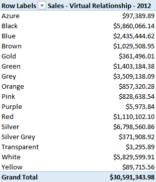
The aggregation of products having the same color is made by the formula engine, which also applies an internal loop to execute the CONTAINS function. This is the same logic used by a PivotTable displaying the following result:

In Power BI and Analysis Services 2017, you can use the TREATAS function to apply the same pattern, as in the following example:
[Sales - Virtual Relationship - 2017] :=
CALCULATE (
    SUMX ( Sales, Sales[Net Price] * Sales[Quantity] ),
    TREATAS (
        VALUES ( 'Product'[ProductKey] ),
        Sales[ProductKey]
    )
)
This is the generic pattern of a virtual relationship using TREATAS:
[Filtered Measure] :=
CALCULATE (
    <target_measure>,
    TREATAS (
        VALUES ( <lookup_granularity_column> ).
        <target_granularity_column>
    )
)
Whenever possible, you should use TREATAS to implement the virtual relationship for performance reasons. If TREATAS is not available, then you can use INTERSECT, which has been introduced in Excel 2016 and Analysis Services 2016. You can use the INTERSECT function to apply the same pattern:
[Sales - Virtual Relationship - 2016] :=
CALCULATE (
    SUMX ( Sales, Sales[Net Price] * Sales[Quantity] ),
    INTERSECT (
        ALL ( Sales[ProductKey] ),
        VALUES ( 'Product'[ProductKey] )
    )
)
In practice, you can apply the following pattern:
[Filtered Measure] :=
CALCULATE (
    <target_measure>,
    INTERSECT (
        ALL ( <target_granularity_column> ),
        VALUES ( <lookup_granularity_column> )
    )
)
The result produced to the user is identical, and the formula engine requires the same data to the storage engine. Thus, you still pay a higher price compared to the query plan obtained using a physical relationship, but the pressure on the formula engine is reduced thanks to a shorter query plan.
As usual, performances considerations are related to specific versions of the engine and could change in the future. You should always analyze the query plan and we might imagine that further optimization will be possible in the future using the INTERSECT pattern.
In the example you can download you will find files for Excel and Power BI. Please note that the use of INTERSECT in Excel 2016 might not work because of possible bugs in the engine that have been already fixed in Analysis Services Tabular 2016 and Power BI Desktop. It will probably work in an upcoming update of Excel 2016.
UPDATE 2018-08-15: An additional technique to propagate a virtual relationship is available with TREATAS, described in the article Propagate filters using TREATAS in DAX.
Treats the columns of the input table as columns from other tables. For each column, filters out any values that are not present in its respective output column.
TREATAS ( <Expression>, <ColumnName> [, <ColumnName> [, … ] ] )
Evaluates an expression in a context modified by filters.
CALCULATE ( <Expression> [, <Filter> [, <Filter> [, … ] ] ] )
Returns TRUE if there exists at least one row where all columns have specified values.
CONTAINS ( <Table>, <ColumnName>, <Value> [, <ColumnName>, <Value> [, … ] ] )
Returns the rows of left-side table which appear in right-side table.
INTERSECT ( <LeftTable>, <RightTable> )
 Marco Russo