 Marco Russo & Alberto Ferrari
Although you can create composite models in multiple different ways, for the sake of simplicity we refer here to the most common scenario; that is, a scenario where you start from a report live connected to a Power BI dataset, and you transform it into a composite model. When the transformation takes place, you gain the capability to extend the original model with new tables and calculations. You end up having two different data models:
- The remote model, which is the original model to which you were live connected and that is transformed into a DirectQuery connection in a local model.
- The local VertiPaq model, created as part of the transformation of the live connected report into a composite model, which includes a DirectQuery connection to the originally live connected dataset.
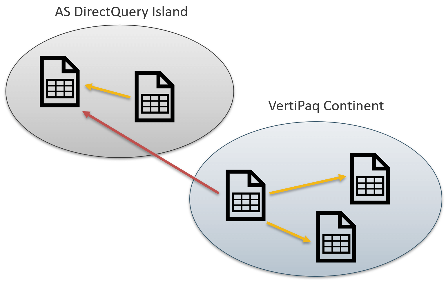
In more technical terms, we say that there are now two data islands: one is the DirectQuery connection with the remote model, the other is the local VertiPaq database that we call the VertiPaq continent. The distinction between continent and island is useful because you can create a solution with multiple DirectQuery islands, but there can only be one VertiPaq continent.
Despite the increased complexity of the storage, the composite model is still a single model. You are free to mix remote and local tables in a DAX query in order to obtain your result. This leaves to Power BI the task of finding a way to separate the queries between local and remote servers.
Nonetheless, it is important to understand how a DAX query is resolved, because this has profound implications on both the speed of the query and the semantics of DAX. The goal of this article is not to analyze performance or semantics, as these topics are covered in other articles. Here, the focus is on understanding the difference between the two ways a query can be executed: wholesale or retail.
A query is wholesale when it uses only tables belonging to either one data island or the continent. The query is retail when it uses data belonging to different islands, or mixes data from the continent and one or more islands.
A wholesale query can be entirely executed by either the remote server, or the local Tabular engine. There is no need to transfer information between different servers. A retail query on the other hand relies on data present in different islands. As such, it is necessary to either send information to the remote server to let it process the query, or to retrieve information from the remote server to process the DAX code locally. Consequently, retail queries are much more complex to optimize: there are at least two different DAX engines involved, with the additional complexity of the size of the data structures that need to be moved back and forth between the two servers.
Moreover, there are scenarios where wholesale calculations are a must. For example, calculated columns on remote tables can be created only if their execution is wholesale. Indeed, calculated columns on remote tables are executed by the remote server through the DEFINE COLUMN clause, which must be executed on the remote server.
Let us elaborate on the concept with a few examples. Imagine we want to cluster sales based on the discount percentage. This can be achieved with two calculated columns, one to compute the discount category and another to compute the discount category sort:
--
--  Calculated column in Sales, sorted by Sales[Discount Category Sort]
--
Discount Category =
VAR DiscountPct = DIVIDE ( Sales[Unit Price] - Sales[Net Price], Sales[Unit Price] )
VAR DiscountCat =
    SWITCH (
        TRUE (),
        DiscountPct = 0, "NO DISCOUNT",
        DiscountPct < 0.05, "LOW DISCOUNT",
        DiscountPct < 0.10, "MEDIUM DISCOUNT",
        "HIGH DISCOUNT"
    )
RETURN
    DiscountCat

--
--  Calculated column in Sales
--
Discount Category Sort =
VAR DiscountPct = DIVIDE ( Sales[Unit Price] - Sales[Net Price], Sales[Unit Price] )
VAR DiscountCatSort =
    SWITCH (
        TRUE (),
        DiscountPct = 0, 0,
        DiscountPct < 0.05, 1,
        DiscountPct < 0.10, 2,
        3
    )
RETURN
    DiscountCatSort
You can create the two columns, because they access only the Sales table. As such, their execution is wholesale, and you can use them in a report.

You can check that the execution is wholesale by inspecting the query generated by Power BI. You do this by using the performance analyzer. The local engine executes this query:
--
--  DAX query executed on the local server to return the visual
--
EVALUATE
SUMMARIZECOLUMNS (
    ROLLUPADDISSUBTOTAL (
        ROLLUPGROUP ( 'Sales'[Discount Category], 'Sales'[Discount Category Sort] ),
        "IsGrandTotalRowTotal"
    ),
    "Sales_Amount", 'Sales'[Sales Amount]
)
Beware that this is just the local query. The local query is transformed into another DAX query sent to the remote server to compute the result. The query sent to the remote server is the following:
--
--  DAX DirectQuery query executed on the remote server
--
DEFINE
    COLUMN 'Sales'[ASDQ_Discount Category Sort] =
        VAR ASDQ_DiscountPct =
            DIVIDE ( Sales[Unit Price] - Sales[Net Price], Sales[Unit Price] )
        VAR ASDQ_DiscountCatSort =
            SWITCH (
                TRUE (),
                ASDQ_DiscountPct = 0, 0,
                ASDQ_DiscountPct < 0.05, 1,
                ASDQ_DiscountPct < 0.10, 2,
                3
            )
        RETURN
            ASDQ_DiscountCatSort
    COLUMN 'Sales'[ASDQ_Discount Category] =
        VAR ASDQ_DiscountPct =
            DIVIDE ( Sales[Unit Price] - Sales[Net Price], Sales[Unit Price] )
        VAR ASDQ_DiscountCat =
            SWITCH (
                TRUE (),
                ASDQ_DiscountPct = 0, "NO DISCOUNT",
                ASDQ_DiscountPct < 0.05, "LOW DISCOUNT",
                ASDQ_DiscountPct < 0.10, "MEDIUM DISCOUNT",
                "HIGH DISCOUNT"
            )
        RETURN
            ASDQ_DiscountCat

EVALUATE
SUMMARIZECOLUMNS (
    ROLLUPADDISSUBTOTAL (
        ROLLUPGROUP (
            'Sales'[ASDQ_Discount Category],
            'Sales'[ASDQ_Discount Category Sort]
        ),
        "IsGrandTotalRowTotal"
    ),
    "Sales_Amount", [Sales Amount]
)
The remote server receives the DirectQuery DAX query and it produces the result. The result of the DirectQuery DAX query is received by the local server, which uses it to produce the result displayed on the visual.
You can manually execute the latter query on the remote server to check the result.

The two servers communicate this way:
- The local server sends the DirectQuery DAX query to the remote server.
- The remote server sends back the result consisting of only 5 rows.
The local server is acting only as a pass-through. It is responsible for translating the local query into a remote query. The result is obtained by the remote server, as is always the case with wholesale calculations.
Things are different when you combine data from different tables. For example, we can improve this solution with a data-driven approach by storing the boundaries of the categories in a local table:
Discount Category =
SELECTCOLUMNS (
    {
        ( 0, "NO DISCOUNT", 0 ),
        ( 1, "LOW DISCOUNT", 0.05 ),
        ( 2, "MEDIUM DISCOUNT", 0.10 ),
        ( 3, "HIGH DISCOUNT", 1 )
    },
    "Discount Code", [Value1],
    "Discount Category", [Value2],
    "Discount Pct", [Value3]
)
If you try to create a data-driven calculated column in Sales that takes advantage of this local table to compute the Discount Code to later build a relationship between the two tables, the result is an error. Indeed, the newly calculated column would not be wholesale:
Discount Category (Data Driven) =
VAR DiscountPct =
    DIVIDE (
        Sales[Unit Price] - Sales[Net Price],
        Sales[Unit Price]
    )
VAR HigherCategories =
    FILTER (
        'Discount Category',
        'Discount Category'[Discount Pct] >= DiscountPct
    )
VAR DiscountCategoryCode =
    MINX (
        HigherCategories,
        'Discount Category'[Discount Code]
    )
RETURN
    DiscountCategoryCode
Indeed, the Discount Category (Data Driven) calculated column should scan the Discount Category table that is stored in the VertiPaq continent. Nonetheless, being a calculated column it must be wholesale and executed by the remote DAX engine. Because the remote model does not have access to the local VertiPaq continent, Power BI returns this error:
The column 'Sales'[Discount Category (Data Driven)] cannot be pushed
to the remote data source and cannot be used in this scenario.
The code of the column cannot be pushed to the remote data source – in other words, it is not wholesale, it is retail. Therefore, it cannot be used in a calculated column.
Retail code cannot be used in calculated columns, but it can be used in measures and in calculated tables. Therefore, a solution to the previous problem is to change the local model. Instead of just creating a table with the four categories, we can expand the table by adding each possible value of the discount percentage, along with the category it belongs to. Then, we can create a calculated column in Sales that only computes the discount percentage and use that column to setup the relationship.
We create a new DiscountPct column in the Sales table to compute the discount percentage, and we then use that column to build the Discount Category Expanded calculated table:
--
-- Calculated column in the Sales table
--
DiscountPct =
    ROUND (
        DIVIDE (
            Sales[Unit Price] - Sales[Net Price],
            Sales[Unit Price]
        ),
        2
    )

--
-- Calculated table
--
Discount Category Expanded =
GENERATE (
    ALLNOBLANKROW ( Sales[DiscountPct] ),
    VAR HigherCategories =
        FILTER (
            'Discount Category',
            'Discount Category'[Discount Pct] >= Sales[DiscountPct]
        )
    VAR DiscountCategoryCode =
        TOPN ( 1, HigherCategories, 'Discount Category'[Discount Code], ASC )
    RETURN
        DiscountCategoryCode
)
Discount Category Expanded can be used to create a relationship because it contains one row for each possible value of DiscountPct. The code of the calculated table mixes local and remote tables in the same expression; therefore, it is necessarily retail. It works in this case because there is no requirement for calculated tables to be wholesale: they can be retail.
Here is the content of Discount Category Expanded.

We can now create the relationship between Sales and Discount Category Expanded.

Despite looking simple, this diagram is actually showing an incredible level of complexity. Indeed, we created a calculated column on the remote island that is actually not a real column: the calculated column on the remote island is computed for every query. Then, we created a calculated table stored in the VertiPaq continent, starting from that very calculated column in the remote island. Finally, we are building a relationship between the calculated column and the calculated table. As you might think, querying such a complex model is not going to be wholesale.
Indeed, the code executed to obtain the following report is much more complex.
This is the local query:
EVALUATE
SUMMARIZECOLUMNS (
    ROLLUPADDISSUBTOTAL (
        ROLLUPGROUP (
            'Discount Category Expanded'[Discount Category],
            'Discount Category Expanded'[Discount code]
        ),
        "IsGrandTotalRowTotal"
    ),
    "Sales_Amount", 'Sales'[Sales Amount]
)
There are now multiple DirectQuery DAX queries:
--
--  This is a first DirectQuery DAX query executed on the remote server
--
DEFINE
    TABLE _T84 =
        UNION (
            SELECTCOLUMNS ( _Var0, "Value", [Value2] ),
            SELECTCOLUMNS ( _Var1, "Value", [Value2] )
        )
    TABLE _T85 =
        UNION (
            SELECTCOLUMNS ( _Var0, "Value", [Value1] ),
            SELECTCOLUMNS ( _Var1, "Value", [Value1] )
        )
    COLUMN 'Sales'[ASDQ_DiscountPct] =
        ROUND ( DIVIDE ( Sales[Unit Price] - Sales[Net Price], Sales[Unit Price] ), 2 )
    VAR _Var0 = { ( 3, 3 ), ( 4, 4 ), ( 5, 5 ), ( 6, 6 ) }
    VAR _Var1 = {
        ( 3, 3, 0 ),
        ( 4, 4, 1.E-2 ),    ( 4, 4, 2.E-2 ),      ( 4, 4, 3.E-2 ),    ( 4, 4, 4.E-2 ),
        ( 4, 4, 5.E-2 ),    ( 5, 5, 6.E-2 ),      ( 5, 5, 7.E-2 ),    ( 5, 5, 8.E-2 ),
        ( 5, 5, 9.E-2 ),    ( 5, 5, 1.E-1 ),      ( 6, 6, 1.1E-1 ),   ( 6, 6, 1.2E-1 ),
        ( 6, 6, 1.3E-1 ),   ( 6, 6, 1.4E-1 )
    }

EVALUATE
GROUPCROSSAPPLYTABLE (
    _T85[Value],
    _T84[Value],
    TREATAS ( _Var0, _T85[Value], _T84[Value] ),
    "L1",
        CALCULATETABLE (
            GROUPCROSSAPPLY (
                TREATAS (
                    DEPENDON (
                        _Var1,
                        EARLIER ( _T85[Value], 1 ),
                        EARLIER ( _T84[Value], 1 )
                     ),
                    'Sales'[ASDQ_DiscountPct]
                ),
                "__Agg0", [Sales Amount]
            ),
            ALL ( _T85[Value] ),
            ALL ( _T84[Value] )
        )
)

--
--  Second DirectQuery DAX query executed on the remote server
--
EVALUATE
GROUPCROSSAPPLY ( "__Agg0", [Sales Amount] )
The DAX code generated is now much more complex. Besides, there are also xmSQL queries executed before these DAX queries, and the formula engine shows the usage of data caches from multiple islands being aggregated together to produce the result of the entire query.
The result of the first DirectQuery DAX query is only partial: even though we aggregate by Discount Category – which is a string – the result contains numbers that the formula engine will then link to string descriptions.

Conclusions
There would be a lot more considerations to perform about this simple example. Nonetheless, this is an introductory article, which is why it does not explain in depth the behavior of DirectQuery DAX queries. The goal here is only to introduce the difference between wholesale and retail executions of DAX code. As you have seen, composite models show a level of complexity much higher than normal models. The simple fact that data can reside in different islands and that the engine must send queries to the remote server increases the challenge of writing good DAX code.
Articles in the Composite model series
- New composite models in Power BI: A milestone in Business Intelligence
- Introducing wholesale and retail execution in composite models
- Understanding the interactions between composite models and calculation groups
- Using ALLSELECTED in composite models