 Marco Russo & Alberto Ferrari
When looking at a report, it is natural to double-check the numbers produced. The simplest and most intuitive way is to verify whether the total equals the sum of individual rows. This behavior is extremely natural and mostly effective. Nonetheless, the total is the sum of rows only for additive measures, which are measures that are naturally computed as a sum.
When working with business intelligence solutions, sooner or later a developer will author a calculation that is non-additive. At that point, the total can no longer be computed by summing the rows for a very good reason: it would be inaccurate. When users complain about the fact that the rows do not sum up, seasoned BI developers offer a rational explanation of the reasons why the number are not summed: this process often provides a better understanding of how values are computed. Choosing the easy way out of introducing additivity in a naturally non-additive calculation means losing the opportunity to generate accurate calculations, and relying on inaccurate values.
Let us start with a very simple report that shows the issue at hand. We want to produce a report that shows the sales amount and the number of products sold on different continents. The two measures are:
Sales Amount :=
SUMX ( Sales, Sales[Quantity] * Sales[Net Price] )
# Products :=
DISTINCTCOUNT ( Sales[ProductKey] )
Once projected in a matrix, this is the result.
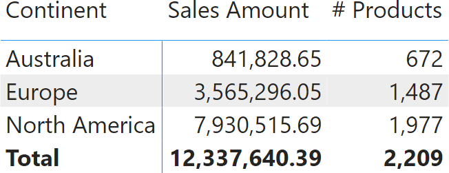
The report clearly shows that Sales Amount is additive: Sales Amount over the entire planet is the sum of sales in each individual continent. Not only it is additive over continents: it is additive over any dimension. The sales amount of all the products is the sum of the sales of each individual product. Same for time: the sales amount in a year is the sum of the sales in each day of that year. Indeed, Sales Amount is a simple additive measure.
The # Products measure behaves differently. You can clearly tell that the value shown at the total level is not the sum of individual rows. The reason is that if the same product is sold in both Australia and Europe, it is counted once in Australia, once in Europe, but only once at the total level. If we were to add individual rows, we would end up with a total showing more products than the ones Contoso sells, like in the following report, where we forced additivity in # Products wrong. This results in an inaccurate report.
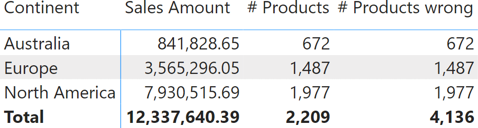
There are not 4,136 products in Contoso’s offering. The total of # Products wrong is – as its name implies – just wrong. By forcing additivity over Customer[Continent], we transformed an accurate measure into an inaccurate measure.
Before moving further, it is worth seeing how we made the formula additive. This is the code of # Products wrong:
# Products wrong :=
SUMX (
    VALUES ( Customer[Continent] ),
    [# Products]
)
To introduce additivity over a column (or a table), we iterate over the values of the column (or the rows of the table) and compute a set of partial results, later aggregated by SUMX. This is a standard pattern that you should learn rather soon on your DAX learning path.
Despite this being only the beginning of the article, a first recap is already useful, because this is an important topic where details are important:
- It does not matter whether a calculation is additive or non-additive. Power BI computes the total by observing what is described in the DAX code and generating an additive (or non-additive) total respecting the developer’s intention.
- A developer can make a non-additive measure additive by introducing an iteration. Sometimes, this is the right thing to do; most often, it is not.
In the specific example we outlined, introducing additivity is not correct. The reason is that forcing the measure to be additive shows the double-counting issue. We do not want to double-count a product, therefore we keep the measure as non-additive, respecting its nature. Be mindful that there is nothing special here. The behavior of Power BI is totally natural. As humans, we easily understand the numbers because distinct counts are intuitively non-additive.
The scenario becomes a bit more complex if, instead of computing a distinct count, we compute the average discount of the transactions in Sales. The Average Discount measure is still simple:
Average Discount :=
AVERAGEX (
    Sales,
    Sales[Quantity] * ( Sales[Unit Price] - Sales[Net Price] )
)
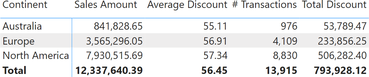
When projected into a matrix, the result shows the average discount of individual sales in dollars.
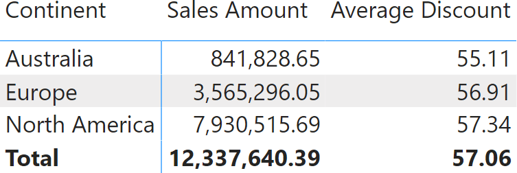
The total of 57.06 is not the average of the values displayed for three continents. Indeed, by doing the math, we discover that 55.11+56.91+57.34 equals 169.36 which divided by three, results in 56.45. Why is Power BI showing 57.06 and not 56.45? Because 56.45 would be inaccurate. Let us discover why.
The number of transactions in each continent is different (# Transactions), and so is the Total Discount expressed in dollars. The larger the number of transactions in a continent, the more relevant the value computed for that continent should be. In the following report, we added the two measures # Transactions and Total Discount, the latter expressed in dollars.
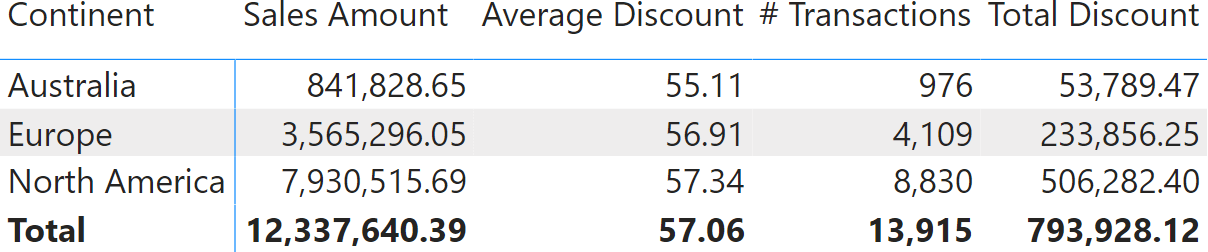
In each row, the average discount is the result of dividing Total Discount by # Transactions. The same goes with the grand total: Total Discount divided by # Transaction equals to Average Discount. The total discount of 57.06 is correct.
Sometimes, users ask for a measure producing a more readable result by averaging individual rows. Nonetheless, the answer is (or should be) always the same: averaging partial results would mean producing the average of an average, which is a different number. The average of an average is rarely the required result. Even though casual users would be happier if they could check the result with a calculator, a business analyst would rather spend time explaining why the result is accurate than allowing an inaccurate number to be produced. An average is non-additive by nature.
At the risk of being pedantic, let us elaborate further on the topic. Let us say that for whatever reason, we want the average discount to be the average of individual rows. We can introduce an iteration over the continent, as we previously did with the # Products measure:
Average Discount :=
AVERAGEX (
    VALUES ( Customer[Continent] ),
    CALCULATE (
        AVERAGEX (
            Sales,
            Sales[Quantity] * (Sales[Unit Price] - Sales[Net Price] )
        )
    )
)
The result is a reassuring (but inaccurate) value of 56.45.
We left the last two columns on purpose: 56.45 can now be explained as the average of displayed Average Discount values, but it can no longer be explained through its most natural interpretation: Total Discount divided by the number of transactions (# Transactions). Nonetheless, things can be worse than this.
Let us say that we switch from slicing by continent to slicing by year.
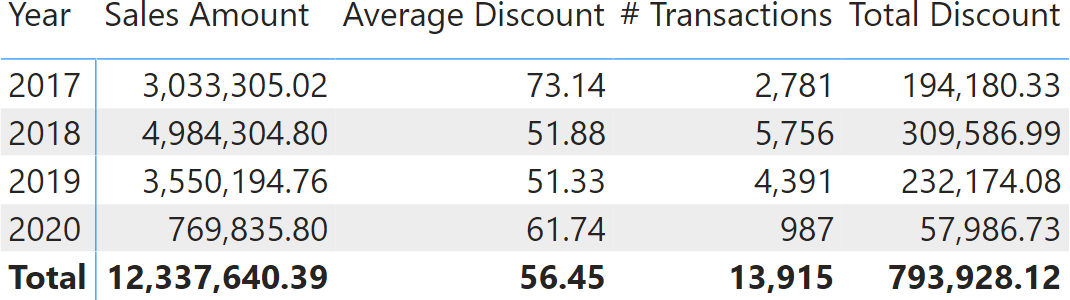
The value shown in the total is still 56.45. However, this time it cannot be explained by looking at any other number in the report. In this report, the average of averages should be 59.52. As a side note, showing 59.52 when browsing by year and 56.45 while browsing by continent would be even more confusing.
The thing is: a measure computing the average is non-additive. As such, it cannot be derived from the values in the rows: it requires a new calculation at the total level.
So far, we analyzed two calculations: a distinct count and an average. Distinct count is clearly non-additive; therefore, we easily accept that it cannot be computed by summing the rows. The average is non-additive too. Nonetheless, we had to elaborate a bit further to show why we need to accept its non-additive nature.
In both scenarios, Power BI did the right thing: it computed the measure at the aggregated level; it did not use the values in the displayed rows to produce some number. The number shown by Power BI has always been the correct number.
Sometimes, additivity is lost because the DAX developer writes inaccurate code. Let us see a simple example of poorly-written code. We created a new measure that shows the number of transactions minus 500. A DAX newbie might write it this way:
# Transactions minus 500 := [# Transactions] – 500
A DAX developer with some experience would immediately spot the problem: the code is mixing together in a subtraction, one value that changes depending on the context and a constant value that represents the same number no matter what the matrix is slicing by. Predictably, the result looks strange.
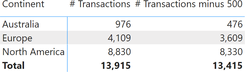
The sum of the three continents for # Transactions minus 500 should be 12,415, not 13,415. The thing is, by using a constant value of 500, we created a non-additive measure. We requested the number of transactions minus 500, no matter what the report is filtering by. In each row, the measure shows the number of transactions minus 500. At the total level, it shows the number of transactions minus 500. Exactly what we asked for. Why isn’t it showing 12,415? Because we did not ask for that. We asked the number of transactions minus 500, and that is what we obtained.
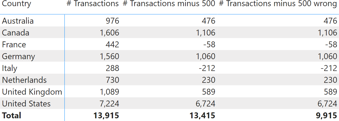
There is a very good reason for this behavior. The value at the grand total level is 13,415 – no matter what the report is slicing by. What number would you expect if instead of slicing by Continent, we were slicing by Country? Here is the result.
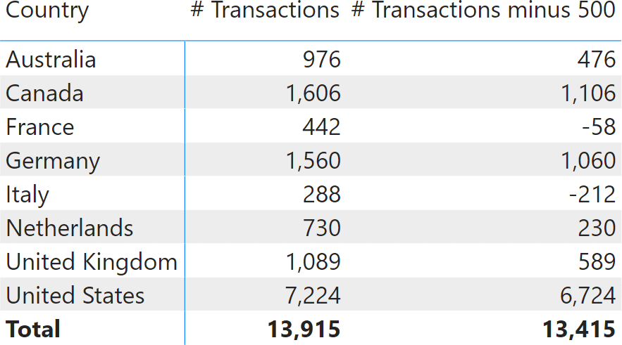
This time, the number seems even worse. There are eight countries; by summing the values by country we obtain 9,915. Instead, the result is still 13,415. If you create a non-additive calculation and then compute it by summing individual rows, then the number changes depending on the column used to slice by. We can double check this in the next example, where we included Transactions minus 500 wrong, which forces additivity over the country:
Transactions Minus 500 wrong :=
SUMX (
    VALUES ( Customer[Country] ),
    [# Transactions] – 500
)
As you see, forcing additivity on a non-additive measure mostly creates inaccurate results. Power BI does not force the additivity of the results displayed because it would produce inaccurate values.
Now that we have covered pieces of theory, let us analyze a more practical example. We want to author a measure that computes Sales Amount for countries where sales exceed 1,000,000. The first, wrong attempt is the following:
Sales GT 1M :=
IF (
    [Sales Amount] >= 1000000, [Sales Amount]
)
The measure works fine at the row level, but if fails at the grand total, showing an inaccurate result.
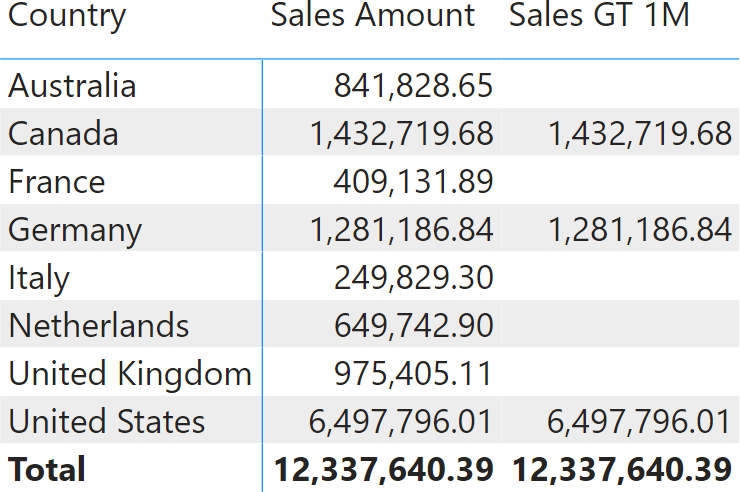
At first glance, it looks like Power BI does not know how to sum numbers. However, we learned that the problem is not in Power BI; it most likely is in the code we authored. The requirement was to show sales for the countries where the amount exceeds 1,000,000. In the DAX code there are no references to the concept of country. We are clearly missing something.
Indeed, because the calculation needs to happen at the country level, we need to change the DAX code to an iteration over countries. We check the condition country by country, and then we sum the values computed at the country level to produce the grand total. The correct formula is the following:
Sales GT 1M :=
SUMX (
    VALUES ( Customer[Country] ),
    IF (
        [Sales Amount] >= 1000000, [Sales Amount]
    )
)
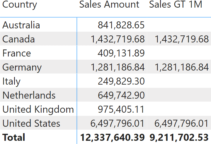
The formula now reflects the requirement in full. Indeed, when used in a report, Sales GT 1M shows the correct total.
The more you advance in your Business Intelligence career, the more non-additive calculations will appear in your projects. Whenever a measure is non-additive, the solution is not to force additivity in some naive way. You need to spend time with the users to understand at which granularity the measure should be computed and then perform an iteration at the correct granularity, summing up the values only later.
Non-additivity is a complex topic. In this article, we just scratched the surface. However, a basic level of experience is enough to discover that whenever Power BI shows an inaccurate total, it is because we authored a non-additive calculation. The solution is always the same: spend some time to refine the measure, check the requirements, and author DAX code that will work in any report.
Returns the sum of an expression evaluated for each row in a table.
SUMX ( <Table>, <Expression> )