Introducing window functions in DAX

INDEX, OFFSET, and WINDOW are new table functions that aim to navigate over a sorted and partitioned table to obtain both absolute and relative rows. The primary purpose of window functions is to make it easier to perform calculations like:

Sorting products by sales amount and comparing the sales of the current product with the previous product.
Comparing the sales in the current month with the previous month.
Finding the difference in the net price of a product between one sale and the previous sale.
Computing moving averages in a window of n months or days.

Window functions by themselves do not increase the expressivity of DAX. Most if not all of the calculations performed with window functions can be expressed with more complex DAX code. The goal is to simplify authoring these calculations and improve their performance.

These new functions also introduce a new concept to the DAX language: “apply semantics”. We will publish more articles about window functions and “apply semantics” over time. SQLBI+ subscribers will get a dedicated video course later this year and already have access to the window functions whitepaper we are currently writing.

Several arguments are common in all the windows functions: we introduce ORDERBY and PARTITIONBY in INDEX, without repeating them in OFFSET and WINDOW. This article aims to introduce the syntax of the new functions rather than providing specific use cases – we will do that in future articles.

Introducing INDEX

INDEX returns the n^th row of a table. For example, if you want to retrieve the best-seller out of your products, you can rely on INDEX with the following code:

EVALUATE
VAR BrandsAndSales =
    ADDCOLUMNS (
        ALL ( 'Product'[Brand] ),
        "@Sales", [Sales Amount]
    )
RETURN
    INDEX (
        1,
        BrandsAndSales,
        ORDERBY ( [@Sales], DESC )
    )

Brand	@Sales
Adventure Works	2,761,057.66

The BrandAndSales variable contains all the product brands with a new @Sales column representing the sales amount.

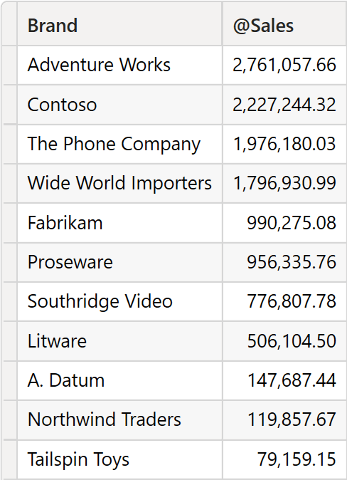
Although we represented the table sorted by @Sales to make it easier to read the article, the variable is not sorted. INDEX requires as its first argument, the position to find; the second argument is the source table, and the third argument is the sorting to use to determine the position. The syntax we use is the following:

DAX Snippet code

 
INDEX ( 
    1, 
    BrandsAndSales, 
    ORDERBY ( 
        [@Sales], 
        DESC 
    ) 
)

Meaning: we want the first row of the BrandsAndSales table after @Sales has sorted it in descending order.

If we are interested in the second-best selling product, it is enough to change the index position to 2; the result is Contoso:

EVALUATE
VAR BrandsAndSales =
    ADDCOLUMNS (
        ALL ( 'Product'[Brand] ),
        "@Sales", [Sales Amount]
    )
RETURN
    INDEX (
        2,
        BrandsAndSales,
        ORDERBY ( [@Sales], DESC )
    )

Brand	@Sales
Contoso	2,227,244.32

The first argument of INDEX can be a positive or a negative number. A positive number indicates the position of the row starting from the beginning (where 1 is the first row of the sorted table). In contrast, a negative number indicates the position of the row starting from the end of the source table (where -1 is the last row of the sorted table).

Handling ties

INDEX requires each row in the input table to be unique. If there are not enough columns in the ORDERBY to guarantee each row is unique, then INDEX automatically adds other columns to the ORDERBY clause to guarantee each row is unique. If the operation cannot be completed (as the input table may contain duplicates), then INDEX fails. When the source table is a reference to a model table, unique rows must be guaranteed through a primary key.

Let us see the behavior with an example. We use the query from before, this time by rounding the value of @Sales to 1 million in order to introduce duplicates:

EVALUATE
VAR BrandsAndSales =
    ADDCOLUMNS (
        ALL ( 'Product'[Brand] ),
        "@Sales",
            MROUND (
                [Sales Amount],
                1E6
            )
    )
RETURN
    INDEX (
        2,
        BrandsAndSales,
        ORDERBY ( [@Sales], DESC )
    )

Brand	@Sales
Contoso	2,000,000

This time, BrandsAndSales contains several rows with the same value for the @Sales column.

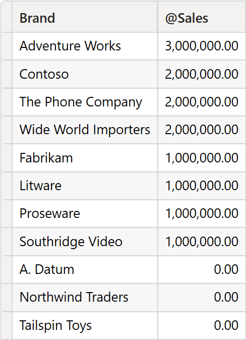
If we were to retrieve the second position, this would be a tie including Contoso, The Phone Company, and Wide World Importers. However, INDEX returns only one row: Contoso.

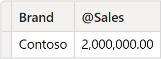
To return a single row, INDEX added the Product[Brand] column to the ORDERBY section. Indeed, each row becomes unique by considering the brand among the sorting columns. Therefore, INDEX can return its result. The same result can be explicitly obtained by using this code:

DAX Snippet code

INDEX (
    2,
    BrandsAndSales,
    ORDERBY ( 
        [@Sales], DESC, 
        Product[Brand], ASC 
    )
)

The way INDEX chooses the columns to add to the ORDERBY section to guarantee rows are unique is not documented. Therefore, there is no way to predict how this is guaranteed. However, it is deterministic, meaning that INDEX does not return a random row: it will always be the same row, even though a developer cannot predict which row it will be. If more determinism is needed, then it is enough to explicitly list all the required columns in the ORDERBY section to drive the algorithm to satisfy our requirements.

Introducing blank handling

INDEX accepts an optional argument to define how to sort blank values. At the time of writing, this optional argument can only be KEEP, meaning that blanks are sorted depending on the column’s datatype: for numbers, they are placed before zero but after any negative number. For strings, they are placed before empty strings – that is, at the top of the sort order.

This optional argument can be skipped, and by default it is KEEP.

Introducing PARTITIONBY

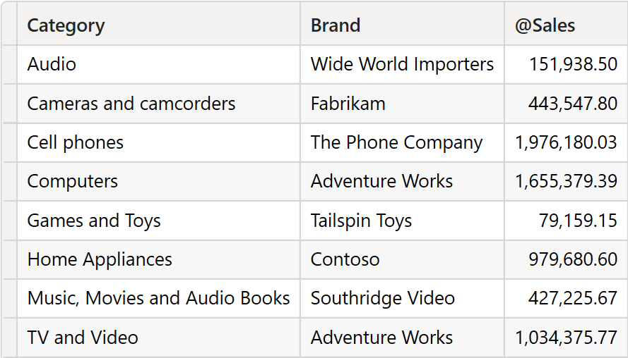
The last argument of INDEX defines how to partition the table. For example, to find the best-selling brand by category, this is the syntax we need:

EVALUATE
VAR BrandsAndSalesByCategory =
    ADDCOLUMNS (
        ALL (
            'Product'[Category],
            'Product'[Brand]
        ),
        "@Sales", [Sales Amount]
    )
RETURN
    INDEX (
        1,
        BrandsAndSalesByCategory,
        ORDERBY ( [@Sales], DESC ),
        KEEP,
        PARTITIONBY ( 'Product'[Category] )
    )

Product[Category]	Product[Brand]	@Sales
Audio	Wide World Importers	151,938.50
TV and Video	Adventure Works	1,034,375.77
Computers	Adventure Works	1,655,379.39
Cameras and camcorders	Fabrikam	443,547.80
Cell phones	The Phone Company	1,976,180.03
Music, Movies and Audio Books	Southridge Video	427,225.67
Games and Toys	Tailspin Toys	79,159.15
Home Appliances	Contoso	979,680.60

BrandsAndSalesByCategory contains three columns.

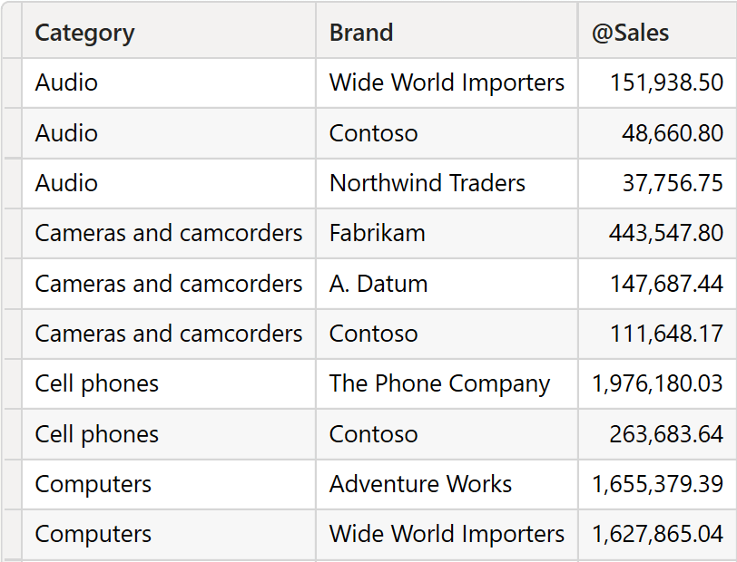
PARTITIONBY instructs INDEX to split the input table by Product[Category] and to compute a local index by category. Therefore, there will be multiple rows indexed as 1: one for Audio, one for Cameras and camcorders, and so on. The result of the query contains the best-selling brand for each category.

Be mindful that this behavior is due to “apply semantics”, a rather advanced and new concept described in the SQLBI+ whitepaper. INDEX, by itself, is designed to return only one row for the current partition; “apply semantics” does the magic and makes it work when multiple current rows exist.

Omitting the source table

In window functions, the source table can be omitted. In that case, its default value is ALLSELECTED over all the columns specified in the ORDERBY section. For example, in the following code, the Sales First Year column is computed using INDEX as a CALCULATE filter specifying only the ORDERBY section:

EVALUATE
SUMMARIZECOLUMNS (
    Product[Brand],
    'Date'[Year],
    "Sales", [Sales Amount],
    "Sales First Year",
        CALCULATE (
            [Sales Amount],
            INDEX (
                1,
                ORDERBY ( 'Date'[Year] )
            )
        )
)

Product[Brand]	Date[Year]	Sales	Sales First Year
Contoso	2,017	511,810.85	511,810.85
Contoso	2,018	868,179.21	511,810.85
Contoso	2,019	707,010.55	511,810.85
Contoso	2,020	140,243.70	511,810.85
Wide World Importers	2,017	483,427.60	483,427.60
Wide World Importers	2,018	737,726.73	483,427.60
Wide World Importers	2,019	458,943.97	483,427.60
Wide World Importers	2,020	116,832.70	483,427.60
Northwind Traders	2,017	21,598.14	21,598.14
Northwind Traders	2,018	64,737.97	21,598.14
…	…	…	…

Because the source table for INDEX is not provided, it defaults to ALLSELECTED ( ‘Date'[Year] ). As such, INDEX returns the first year, and CALCULATE computes the sales in the first year.

Introducing OFFSET

OFFSET returns a row relative to the current row. OFFSET receives as the first argument the number of rows to move back or forth, then it receives the source table, and then the usual ORDERBY and PARTITIONBY sections to define the sorting of rows.

For example, the following query returns the dates with sales, and with no sales the day before. Because the result is always a single row, we used SELECTCOLUMNS in the definition of the PreviousDate variable to extract the column of interest. The result contains the dates and the sales amount on that date:

EVALUATE
VAR DatesAndSales =
    FILTER (
        ADDCOLUMNS (
            ALL ( 'Date'[Date] ),
            "@Sales", [Sales Amount]
        ),
        [@Sales] > 0
    )
RETURN
    SELECTCOLUMNS (
        FILTER (
            DatesAndSales,
            VAR CurrentDate = 'Date'[Date]
            VAR PreviousDate =
                SELECTCOLUMNS (
                    OFFSET (
                        -1,
                        DatesAndSales,
                        ORDERBY ( 'Date'[Date], ASC )
                    ),
                    'Date'[Date]
                )
            RETURN
                PreviousDate <> CurrentDate - 1
        ),
        "Date", 'Date'[Date],
        "Sales Amount", [@Sales]
    )

Date	Sales Amount
2017-05-18	43,369.49
2017-05-22	10,896.70
2017-05-29	5,531.21
2017-06-05	5,921.99
2017-06-12	8,084.23
2017-06-19	3,874.36
2017-06-26	2,460.79
2017-07-03	20,826.45
…	…

When using OFFSET, developers should pay special attention to the filter context of the visual and of the evaluation of OFFSET. An example may be of great help in understanding the issue.

The following code computes the sales in the previous year by using OFFSET. In our model, sales start in 2017, and go up to 2020. The query reports only two years: 2019 and 2020. Quite surprisingly, the Prev Year Sales measure does not report any value:

DEFINE
    MEASURE Sales[Prev Year Sales] =
        CALCULATE (
            [Sales Amount],
            OFFSET (
                -1,
                ORDERBY ( 'Date'[Year], ASC )
            )
        )
EVALUATE
SUMMARIZECOLUMNS (
    'Date'[Year],
    TREATAS ( { 2019, 2020 }, 'Date'[Year] ),
    "Sales Amount", [Sales Amount],
    "Prev Year Sales", [Prev Year Sales]
)

Date[Year]	Sales Amount	Prev Year Sales
2,019	3,550,194.76	(Blank)
2,020	769,835.80	3,550,194.76

The problem is within OFFSET. Because we did not specify the source table, OFFSET automatically generated the table using ALLSELECTED over all the columns specified in ORDERBY. Because of the filter in SUMMARIZECOLUMNS, ALLSELECTED ( Date[Year] ) returns { 2019, 2020 }. When the current row is 2019, as is the case in the first row, there is no previous row to return. As such, OFFSET returns an empty table, and no filtering occurs.

Relying on the automatic table generation can produce simpler code – at the risk of not finding the desired rows, and of obtaining an inaccurate result. The correct way to express the calculation is to extend the filter context of the source table by using ALL ( ‘Date'[Year] ). Using ALL to ignore the previous filters on year produces the correct result:

DEFINE
    MEASURE Sales[Prev Year Sales] =
        CALCULATE ( 
            [Sales Amount], 
            OFFSET ( 
                -1, 
                ALL ( 'Date'[Year] ),
                ORDERBY ( 'Date'[Year], ASC ) 
            ) 
        )

EVALUATE
SUMMARIZECOLUMNS (
    'Date'[Year],
    TREATAS ( { 2019, 2020 }, 'Date'[Year] ),
    "Sales Amount", [Sales Amount],
    "Prev Year Sales", [Prev Year Sales]
)

Date[Year]	Sales Amount	Prev Year Sales
2,019	3,550,194.76	4,984,304.80
2,020	769,835.80	3,550,194.76

Be mindful that using ALL is not considered a best practice with every dimension. Developers need to evaluate what to consider the previous or next row carefully. With the version that we developed using ALL, the definition of the previous row is no longer visual. This is mostly desired when dealing with dates, but there are scenarios where the requirements differ.

Introducing WINDOW

Among the window functions, WINDOW is the most complex one. It allows the definition of a window based on the current row using either relative offsets or absolute references. Moreover, “apply semantics” and WINDOW produce complex results that require even more attention. With complexity comes power. WINDOWS is extremely powerful in computing running totals, moving averages, or complex totals.

INDEX and OFFSET return only one row for a given input row. “Apply semantics” may result in tables with multiple rows. By nature, WINDOWS returns a table with multiple rows. “Apply semantics” may result in WINDOW returning larger tables with the UNION of all the tables evaluated for the “current” rows.

To specify the subset of the source table to return, you provide the boundaries: the table’s first and last indexes. Those indexes can be absolute (e.g. the first row) or relative (e.g. three rows before the current one).

As a first example, let us use WINDOW to compute a moving average of six months:

Measure in Sales table

6 Months Avg =
AVERAGEX (
    WINDOW (
        -5, REL,
         0, REL,
        ORDERBY ( 'Date'[Year Month Number], ASC, 'Date'[Year Month], ASC )
    ),
    [Sales Amount]
)

Once placed in a chart along with the sales amount, you can see that the moving average smoothens the line.

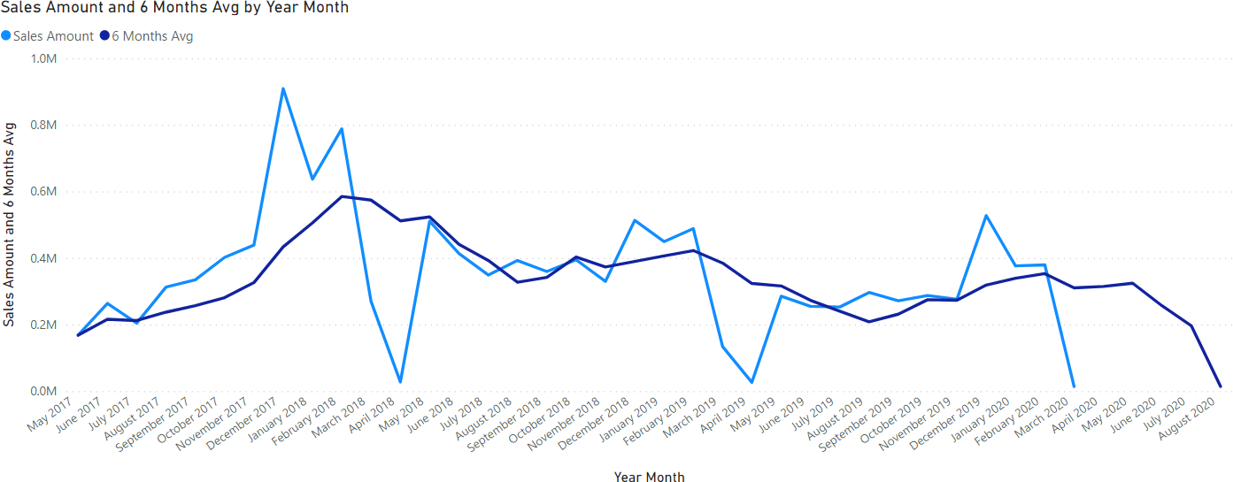
In this code, we used relative offsets. Indeed, the window goes from -5 relative to the current row, up to zero relative to the current row. Therefore, it returns a table containing 6 rows, including the current one.

By computing a window that starts from the first absolute row up to the current one, you can compute a running total. The result accumulates values from the beginning of time up to the current value:

EVALUATE
SUMMARIZECOLUMNS (
    'Date'[Year Month Number],
    'Date'[Year Month],
    "Sales Amount", [Sales Amount],
    "Sales RT",
        SUMX (
            WINDOW (
                1, ABS,
                0, REL,
                ORDERBY ( 
                    'Date'[Year Month Number], ASC,
                    'Date'[Year Month], ASC 
                )
            ),
            [Sales Amount]
        )
)
ORDER BY 'Date'[Year Month Number]

Date[Year Month Number]	Date[Year Month]	Sales Amount	Sales RT
24209	May 2017	168,392.56	168,392.56
24210	June 2017	263,600.69	431,993.25
24211	July 2017	204,281.19	636,274.44
24212	August 2017	312,793.50	949,067.94
24213	September 2017	334,423.50	1,283,491.44
24214	October 2017	402,067.05	1,685,558.49
24215	November 2017	438,804.70	2,124,363.19
24216	December 2017	908,941.83	3,033,305.02
24217	January 2018	636,983.88	3,670,288.90
24218	February 2018	788,062.88	4,458,351.78
24219	March 2018	269,320.40	4,727,672.19
…	…	…	…

WINDOW also works with PARTITIONBY, the same way the other window functions do. For example, to transform the running total into a year-to-date, you only need to partition by Date[Year] to obtain a calculation that is local to the year. As you see, the result now resets in January, and restarts the calculation:

EVALUATE
SUMMARIZECOLUMNS (
    'Date'[Year Month Number],
    'Date'[Year Month],
    "Sales Amount", [Sales Amount],
    "Sales RT",
        SUMX (
            WINDOW (
                1, ABS,
                0, REL,
                ORDERBY ( 
                    'Date'[Year Month Number], ASC,
                    'Date'[Year Month], ASC 
                ),
                PARTITIONBY ( 'Date'[Year] )
            ),
            [Sales Amount]
        )
)
ORDER BY 'Date'[Year Month Number]

Date[Year Month Number]	Date[Year Month]	Sales Amount	Sales RT
24209	May 2017	168,392.56	168,392.56
24210	June 2017	263,600.69	431,993.25
24211	July 2017	204,281.19	636,274.44
24212	August 2017	312,793.50	949,067.94
24213	September 2017	334,423.50	1,283,491.44
24214	October 2017	402,067.05	1,685,558.49
24215	November 2017	438,804.70	2,124,363.19
24216	December 2017	908,941.83	3,033,305.02
24217	January 2018	636,983.88	636,983.88
24218	February 2018	788,062.88	1,425,046.76
24219	March 2018	269,320.40	1,694,367.17
…	…	…	…

Conclusions

In this article, we just scratched the surface of the window function by introducing their syntax and a few simple calculations. Window functions open new possibilities in DAX. Anytime you need to navigate over a sorted table, window functions prove to be fast and easy to author. They require time to get used to, and as is always the case with DAX, they hide some level of complexity with “apply semantics”. Performance requires some attention too. Despite usually being very fast, there are scenarios where more canonical DAX code performs better. We will publish more articles in the future as we learn the best practices for window functions.