Month-related calculations

This pattern describes how to compute month-related calculations such as year-to-date, same period last year, and percentage growth using a month granularity. This pattern does not rely on DAX built-in time intelligence functions.
You can use the Month-related calculations pattern if the analysis over sales is executed at the month level (or above) only. In other words, the formulas stop working if you drill down to the date level. Because the pattern does not use real dates to link to sales, you can also implement fiscal calendars with 13 months and any non-standard time-related calculation – provided that the maximum level of detail of the reports is the month and not weeks or days. The report cannot filter or group by week, day of week, or working days; despite the fact that the granularity of the Date table can be at the date level, these columns must not be part of the Date table because they are not compatible with the formulas in this pattern.
The Month-related calculations pattern is useful to create simple formulas and optimal performance in all those cases where the day granularity is not required. Moreover, this is the only pattern that allows the creation of additional months, like a 13th virtual month for a fiscal year that contains year-end adjustments in accounting systems. If you manage time-related calculations over time periods based on months and you need the day granularity, consider using the Custom time-related calculations pattern. If you manage time-related calculations over time periods based on weeks, consider using the Week-related calculations pattern.
Introduction to month-related time intelligence calculations
The time intelligence calculations in this pattern modify the filter context over the Date table to obtain the result. The formulas are designed to apply filters at the month granularity to improve query performance, regardless of the cardinality of the Date table. For example, many calculations modify the filter context at the month level instead of the individual dates. This technique reduces the cost of computing the new filter and applying it to the filter context. This optimization is especially useful when using DirectQuery, even though it also improves performance on models imported in memory.
The pattern does not rely on the standard time intelligence functions; therefore, the Date table does not have the requirements needed for standard DAX time intelligence functions. The formulas are identical whether you have one row for each month or one row for each day.
If the Date table has a Date column, the Mark as Date Table setting is allowed but not required. The formulas in this pattern do not rely on the automatic REMOVEFILTERS applied over the Date table when the Date column is filtered. Instead, all the formulas use a specific REMOVEFILTERS over the Date table to get rid of the existing filters, in turn replacing them with the minimal number of filters that guarantee the desired result.
Building a Date table
The Date table used for month-related calculations can be built in many ways. The requirement for the pattern is to expose columns related to the months and any aggregation over months, such as quarters and years. The months could be different from those defined in the standard Gregorian calendar, as is the case when a 13th month is required. The sample files available for this pattern include four different scenarios for the Date table:
- One row for each date based on the Gregorian calendar, using Date as the primary key. In this case, the behavior is close to the standard time intelligence calculations, with the noticeable difference that the formulas are faster.
- One row for each month based on the Gregorian calendar, using Year Month Number as the primary key. This pattern is even better than the previous one, because the date table is significantly smaller.
- One row for each month in an accounting calendar with 13 fiscal months, where the 13th fiscal month is projected as an additional month in the Gregorian calendar between the last month of a fiscal year and the first month of the following fiscal year. Performance is close to that of the second pattern.
- One row for each month in an accounting calendar with 13 fiscal months, where the 13th fiscal month is projected in the last fiscal month on the Gregorian calendar. Performance and behavior are very close to what is observed in the third example.
In case there is one row for each month in the Date table, you should not use a date to link the Sales and Date tables – unless you use specific dates to identify each month. For example, December 1 for December and December 31 for the 13th month of the year.
The Date table in this pattern must have all the months included in the range between the first and the last date referenced in the Sales table. Therefore, if the last sale was processed in August 2009, the last month in the Date table must be August 2009. This requirement is different from the requirement of the standard time-intelligence functions in DAX, where all the months of a year must be present in the Date table to guarantee the correct behavior.
If you already have a Date table, you can import the table and use it by showing only the columns required for this pattern while hiding columns with a day or week granularity. If a Date table is not available, you can create one using a DAX calculated table. As an example, the following DAX expression defines the Date table used in the first three scenarios described earlier:
Date =
VAR FirstFiscalMonth = 3   -- First month of the fiscal year
VAR MonthsInYear = 12      -- Must be 12 for GranularityByDate
                           -- can be different for GranularityByMonth
VAR CalendarFirstDate = MIN ( Sales[Order Date]  )
VAR CalendarLastDate = MAX ( Sales[Order Date]  )
VAR CalendarFirstYear = YEAR ( CalendarFirstDate )
VAR CalendarFirstMonth = MONTH ( CalendarFirstDate )
VAR CalendarLastYear = YEAR ( CalendarLastDate )
VAR CalendarLastMonth = MONTH ( CalendarLastDate )

-------------------------
-- Internal calculations
-------------------------
VAR GranularityByDate =
    ADDCOLUMNS (
        CALENDAR (
            DATE ( CalendarFirstYear, CalendarFirstMonth, 1 ),
            EOMONTH (
                DATE ( CalendarLastYear, CalendarLastMonth, 1 ),
                0
            )
        ),
        "Year Month Number", YEAR ( [Date] ) * MonthsInYear
            + MONTH ( [Date] ) - 1
    )
VAR GranularityByMonth =
    SELECTCOLUMNS (
        GENERATESERIES (
            CalendarFirstYear * MonthsInYear + CalendarFirstMonth - 1
                - (MonthsInYear - 12) * (CalendarFirstMonth < FirstFiscalMonth),
            CalendarLastYear * MonthsInYear + CalendarLastMonth - 1
                - (MonthsInYear - 12) * (CalendarLastMonth < FirstFiscalMonth),
            1
        ),
        "Year Month Number", [Value]
    )
RETURN GENERATE (
    GranularityByDate,        -- Use GranularityByMonth to get one row for each month
    VAR YearMonthNumber = [Year Month Number]
    VAR FiscalMonthNumber =
        MOD (
            YearMonthNumber + 1
                * (FirstFiscalMonth > 1)
                * (MonthsInYear + 1 - FirstFiscalMonth),
            MonthsInYear
        ) + 1
    VAR FiscalYearNumber =
        QUOTIENT (
            YearMonthNumber + 1
                * (FirstFiscalMonth > 1)
                * (MonthsInYear + 1 - FirstFiscalMonth),
            MonthsInYear
        )
    VAR OffsetFiscalMonthNumber = MonthsInYear + 1 - (MonthsInYear - 12)
    VAR MonthNumber =
        IF (
            FiscalMonthNumber <= 12 && FirstFiscalMonth > 1,
            FiscalMonthNumber + FirstFiscalMonth
                - IF (
                    FiscalMonthNumber > (OffsetFiscalMonthNumber - FirstFiscalMonth),
                    OffsetFiscalMonthNumber,
                    1
                ),
            FiscalMonthNumber
        )
    VAR YearNumber = FiscalYearNumber - 1 * (MonthNumber > FiscalMonthNumber)
    VAR YearMonthKey = YearNumber * 100 + MonthNumber

    VAR MonthDate = DATE ( YearNumber, MonthNumber, 1 )
    VAR FiscalQuarterNumber = MIN ( ROUNDUP ( FiscalMonthNumber / 3, 0 ), 4 )
    VAR FiscalYearQuarterNumber = FiscalYearNumber * 4 + FiscalQuarterNumber - 1
    VAR FiscalMonthInQuarterNumber =
        MOD ( FiscalMonthNumber - 1, 3 ) + 1 + 3 * (MonthNumber > 12)
    VAR MonthInQuarterNumber = MOD ( MonthNumber - 1, 3 ) + 1 + 3 * (MonthNumber > 12)
    VAR QuarterNumber = MIN ( ROUNDUP ( MonthNumber / 3, 0 ), 4 )
    VAR YearQuarterNumber = YearNumber * 4 + QuarterNumber - 1
    RETURN ROW (
        "Year Month Key", YearMonthKey,
        "Year", YearNumber,
        "Year Quarter", FORMAT ( QuarterNumber, "\Q0" )
            & "-" & FORMAT ( YearNumber, "0000" ),
        "Year Quarter Number", YearQuarterNumber,
        "Quarter", FORMAT ( QuarterNumber, "\Q0" ),
        "Year Month", IF (
            MonthNumber > 12,
            FORMAT ( MonthNumber, "\M00" ) & FORMAT ( YearNumber, " 0000" ),
            FORMAT ( MonthDate, "mmm yyyy" )
        ),
        "Month", IF (
            MonthNumber > 12,
            FORMAT ( MonthNumber, "\M00" ),
            FORMAT ( MonthDate, "mmm" )
        ),
        "Month Number", MonthNumber,
        "Month In Quarter Number", MonthInQuarterNumber,
        "Fiscal Year", FORMAT ( FiscalYearNumber, "\F\Y 0000" ),
        "Fiscal Year Number", FiscalYearNumber,
        "Fiscal Year Quarter", FORMAT ( FiscalQuarterNumber, "\F\Q0" ) & "-"
            & FORMAT ( FiscalYearNumber, "0000" ),
        "Fiscal Year Quarter Number", FiscalYearQuarterNumber,
        "Fiscal Quarter", FORMAT ( FiscalQuarterNumber, "\F\Q0" ),
        "Fiscal Month", IF (
            MonthNumber > 12,
            FORMAT ( MonthNumber, "\M00" ),
            FORMAT ( MonthDate, "mmm" )
        ),
        "Fiscal Month Number", FiscalMonthNumber,
        "Fiscal Month In Quarter Number", FiscalMonthInQuarterNumber
    )
)
You can customize the first two variables to build a Date table that meets specific business requirements. The FirstFiscalMonth variable defines the first fiscal month in the year, and the MonthsInYear variable defines the number of months for each fiscal year. The other customization is the first argument of GENERATE, which can be:
- GranularityByMonth to generate one row for each month;
- GranularityByDate to generate one row for each date.
The GranularityByDate argument is used in the first scenario (one row for every date), whereas GranularityByMonth is used in the other three scenarios (one row for every month). The Year Month column has one value for each month; the month description is the same for both the fiscal and Gregorian calendar hierarchies. The fourth scenario includes a few additional columns to get a different value between Month and Fiscal Month. This is required to manage the 13th month differently, depending on the hierarchy.
In order to obtain the correct visualization, the calendar columns must be configured in the data model as follows. For each column we show the data type followed by a sample value assuming a fiscal month starting in March where there are 12 months in the fiscal year:
- Date: Date, Hidden (8/14/2007), used only for the first scenario
- Year Month Key: Whole Number, Hidden (200708), used to define relationships
- Year Month: Text (Aug 2007)
- Year Quarter: Text (Q3-2007)
- Year Quarter Number: Whole Number, Hidden (8030)
- Quarter: Text (Q3)
- Year Month Number: Whole Number, Hidden (24091)
- Month: Text (Aug)
- Month Number: Whole Number, Hidden (8)
- Month In Quarter Number: Whole Number, Hidden (2)
- Fiscal Month: Text (Aug)
- Fiscal Month Number: Whole Number, Hidden (6)
- Fiscal Month in Quarter Number: Whole Number, Hidden (3)
- Fiscal Year: Text (FY 2008)
- Fiscal Year Number: Whole Number, Hidden (2008)
- Fiscal Year Quarter: Text (FQ2-2008)
- Fiscal Year Quarter Number: Whole Number, Hidden (8033)
- Fiscal Quarter: Text (FQ2)
The Date table in this pattern has four hierarchies:
- Fiscal Year-Quarter: Year (Fiscal Year), Quarter (Fiscal Year Quarter), Month (Year Month)
- Fiscal Year-Month: Year (Fiscal Year), Month (Year Month)
- Year-Quarter: Year (Year), Quarter (Year Quarter), Month (Year Month)
- Year-Month: Year (Year), Month (Year Month)
Several columns serve the only purpose of simplifying the formulas used in custom time-related calculations. The Year Month Key column is only used to define a relationship with the Sales table using an integer in the format YYYYMM. This numeric format to identify a month is common in many data sources that manage data at the month granularity.
The Date table has only the range of months required by the data available. For example, in the example the Date table includes only the months from March 2007 to August 2009. This pattern does not come with the constraint of including all the months in one year. For this reason, there is no need for additional calculated columns like the DateWithSales used in the Standard time-related calculations pattern.
Naming convention
This section describes the naming convention we adopted to reference the time intelligence calculations. A simple categorization shows whether a calculation:
- shifts over a period of time, for example the same period in the previous year;
- performs an aggregation, for example year-to-date; or
- compares two time periods, for example this year compared to last year.
| Acronym | Description | Shift | Aggregation | Comparison |
| YTD | Year-to-date | |||
| QTD | Quarter-to-date | |||
| MAT | Moving annual total | |||
| PY | Previous year | |||
| PQ | Previous quarter | |||
| PM | Previous month | |||
| PYC | Previous year complete | |||
| PQC | Previous quarter complete | |||
| PMC | Previous month complete | |||
| PP | Previous period; automatically selects year, quarter, or month | |||
| PYMAT | Previous year moving annual total | |||
| YOY | Year-over-year | |||
| QOQ | Quarter-over-quarter | |||
| MOM | Month-over-month | |||
| MATG | Moving annual total growth | |||
| POP | Period-over-period; automatically selects year, quarter, or month | |||
| PYTD | Previous year-to-date | |||
| PQTD | Previous quarter-to-date | |||
| YOYTD | Year-over-year-to-date | |||
| QOQTD | Quarter-over-quarter-to-date | |||
| YTDOPY | Year-to-date-over-previous-year | |||
| QTDOPQ | Quarter-to-date-over-previous-quarter |
Computing period-to-date totals
The year-to-date, quarter-to-date, and month-to-date calculations modify the filter context for the Date table, so to include the dates from the beginning of the period to the currently selected month.
Year-to-date total
The year-to-date aggregates data starting from the first day of the year, as shown in Figure 1.
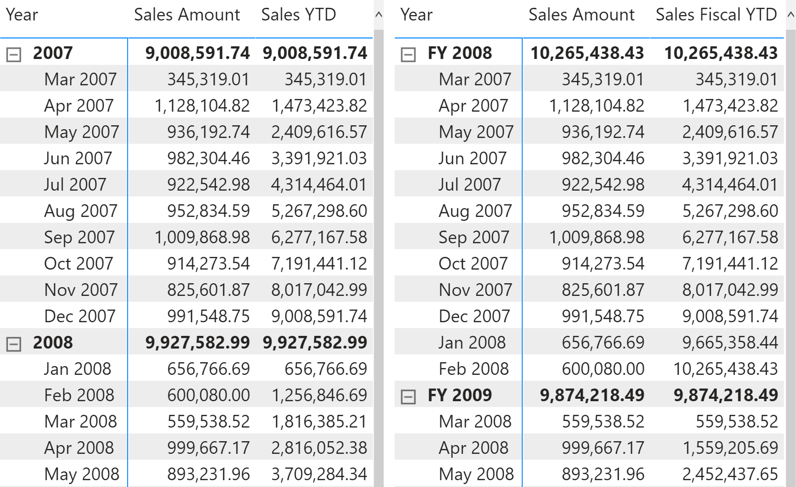
The year-to-date total of a measure filters all the months that are in the year of the last date available in the filter context, and whose month is less than or equal to the month of that date:
Sales YTD :=
VAR LastMonthAvailable = MAX ( 'Date'[Year Month Number] )
VAR LastYearAvailable = MAX ( 'Date'[Year] )
VAR Result =
    CALCULATE (
        [Sales Amount],
        REMOVEFILTERS ( 'Date' ),
        'Date'[Year Month Number] <= LastMonthAvailable,
        'Date'[Year] = LastYearAvailable
    )
RETURN
    Result
If the report uses a hierarchy based on the fiscal year, then the measure must filter the corresponding columns with the word “Fiscal” before the acronym identifying the time intelligence calculation. For example, the Sales Fiscal YTD measure uses Fiscal Year Number instead of Year; however, it does not change the filter over Year Month Number because that column is identical for both fiscal and calendar hierarchies:
Sales Fiscal YTD :=
VAR LastMonthAvailable = MAX ( 'Date'[Year Month Number] )
VAR LastFiscalYearAvailable = MAX ( 'Date'[Fiscal Year Number] )
VAR Result =
    CALCULATE (
        [Sales Amount],
        REMOVEFILTERS ( 'Date' ),
        'Date'[Year Month Number] <= LastMonthAvailable,
        'Date'[Fiscal Year Number] = LastFiscalYearAvailable
    )
RETURN
    Result
Quarter-to-date total
The quarter to date aggregates data from the first month of the fiscal quarter, as shown in Figure 2.
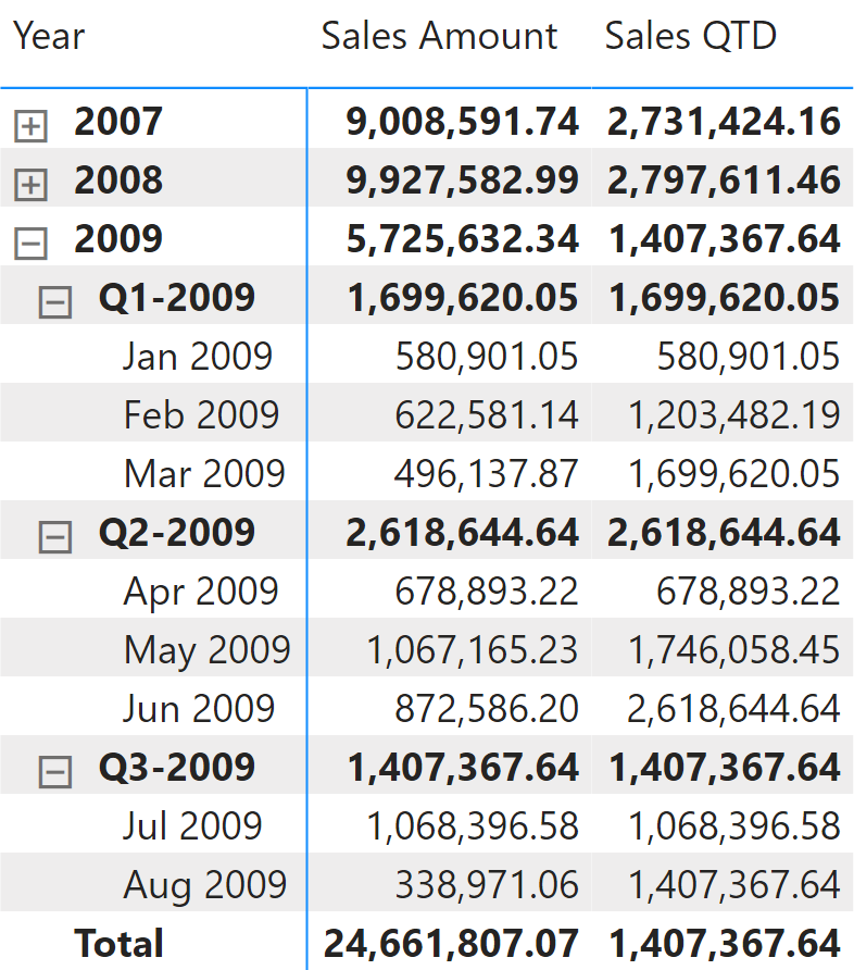
The quarter-to-date total of a measure is computed with the technique used for the year-to-date total. The only difference is that the filter is now on Year Quarter Number instead of Year:
Sales QTD :=
VAR LastMonthAvailable = MAX ( 'Date'[Year Month Number] )
VAR LastYearQuarterAvailable = MAX ( 'Date'[Year Quarter Number] )
VAR Result =
    CALCULATE (
        [Sales Amount],
        REMOVEFILTERS ( 'Date' ),
        'Date'[Year Month Number] <= LastMonthAvailable,
        'Date'[Year Quarter Number] = LastYearQuarterAvailable
    )
RETURN
    Result
Computing period-over-period growth
A common requirement is to compare a time period with the same time period in the previous year, quarter, or month. In order to achieve a fair comparison, the measure takes into account the same relative months in the previous year, or the same relative months in the previous quarter.
Year-over-year growth
Year-over-year compares a time period to its equivalent in the previous year. In this example, data is available until August 2009. For this reason, Sales PY shows numbers related to the year 2009 considering transactions only from before August 2008. Figure 3 shows that the Sales Amount of 2008 is 9,927,582.99, whereas Sales PY for 2009 returns 6,166,534.30 because the measure involves sales only up to August 2008.
Sales PY removes all the filters from the Date table; it filters the Year column by using the previous year, and by using VALUES it retrieves the months visible in the current filter context to then filter the Month Number column. The Date table must hold only the months with sales, instead of holding all the months of the year as required by the standard time intelligence functions in DAX. This way, any direct or indirect selection of months is applied to the previous year:
Sales PY :=
VAR CurrentYearNumber = SELECTEDVALUE ( 'Date'[Year] )
VAR PreviousYearNumber = CurrentYearNumber - 1
VAR Result =
    CALCULATE (
        [Sales Amount],
        REMOVEFILTERS ( 'Date' ),
        'Date'[Year] = PreviousYearNumber,
        VALUES ( 'Date'[Month Number] )
    )
RETURN
    Result
Year-over-year growth is computed as an amount in Sales YOY, and as a percentage in Sales YOY %. Both measures use Sales PY to take into account dates only up to August 2009:
Sales YOY :=
VAR ValueCurrentPeriod = [Sales Amount]
VAR ValuePreviousPeriod = [Sales PY]
VAR Result =
    IF (
        NOT ISBLANK ( ValueCurrentPeriod ) && NOT ISBLANK ( ValuePreviousPeriod ),
        ValueCurrentPeriod - ValuePreviousPeriod
    )
RETURN
    Result
Sales YOY % :=
DIVIDE (
    [Sales YOY],
    [Sales PY]
)
Quarter-over-quarter growth
Quarter-over-quarter compares a time period to its equivalent in the previous quarter. In this example, data is available until August 2009. For this reason, Sales PQ shows numbers related to Q3-2009 considering only transactions before the second month of Q2-2009. Figure 4 shows that the Sales Amount of Q2-2009 is 2,618,644.64, whereas Sales PY for Q3-2009 returns 1,746,058.45. This is because the measure takes into account the sales of only the first two months of Q2-2009.
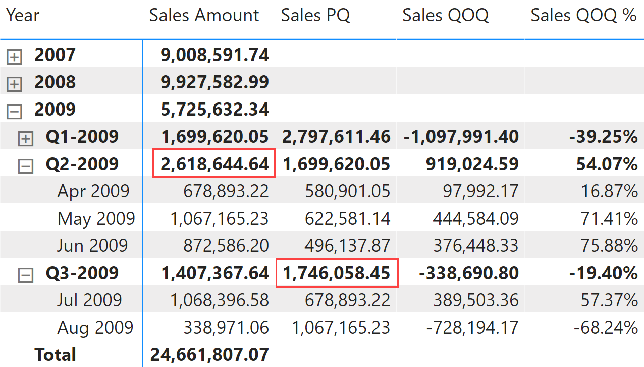
Sales PQ removes all the filters from the Date table; it filters the Year Quarter Number column using the previous quarter, and with VALUES which retrieves the months visible in the filter context it filters the Month In Quarter Number column. This way, any direct or indirect selection of months is applied to the previous quarter:
Sales PQ :=
VAR CurrentYearQuarterNumber = SELECTEDVALUE ( 'Date'[Year Quarter Number] )
VAR PreviousYearQuarterNumber = CurrentYearQuarterNumber - 1
VAR Result =
    CALCULATE (
        [Sales Amount],
        REMOVEFILTERS ( 'Date' ),
        'Date'[Year Quarter Number] = PreviousYearQuarterNumber,
        VALUES ( 'Date'[Month In Quarter Number] )
    )
RETURN
    Result
Quarter-over-quarter growth is computed as an amount in Sales QOQ and as a percentage in Sales QOQ %. Both measures use Sales PQ to guarantee a fair comparison:
Sales QOQ :=
VAR ValueCurrentPeriod = [Sales Amount]
VAR ValuePreviousPeriod = [Sales PQ]
VAR Result =
    IF (
        NOT ISBLANK ( ValueCurrentPeriod )
            && NOT ISBLANK ( ValuePreviousPeriod ),
        ValueCurrentPeriod - ValuePreviousPeriod
    )
RETURN
    Result
Sales QOQ % :=
DIVIDE (
    [Sales QOQ],
    [Sales PQ]
)
Month-over-month growth
Month-over-month compares a time period to its equivalent in the previous month. Figure 5 shows that Sales PM always corresponds to the Sales Amount of the previous month and does not produce any result at the quarter and at the year levels (only the year level is visible in Figure 5).
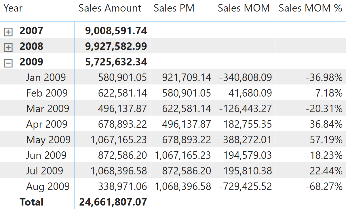
Sales PM removes all the filters from the Date table and only filters the Year Month Number column using the previous month:
Sales PM :=
VAR CurrentYearMonthNumber = SELECTEDVALUE ( 'Date'[Year Month Number] )
VAR PreviousYearMonthNumber = CurrentYearMonthNumber - 1
VAR Result =
    CALCULATE (
        [Sales Amount],
        REMOVEFILTERS ( 'Date' ),
        'Date'[Year Month Number] = PreviousYearMonthNumber
    )
RETURN
    Result
The month-over-month growth is computed as an amount in Sales MOM and as a percentage in Sales MOM %:
Sales MOM :=
VAR ValueCurrentPeriod = [Sales Amount]
VAR ValuePreviousPeriod = [Sales PM]
VAR Result =
    IF (
        NOT ISBLANK ( ValueCurrentPeriod ) && NOT ISBLANK ( ValuePreviousPeriod ),
        ValueCurrentPeriod - ValuePreviousPeriod
    )
RETURN
    Result
Sales MOM % :=
DIVIDE (
    [Sales MOM],
    [Sales PM]
)
Period-over-period growth
Period-over-period growth automatically selects one of the measures previously described in this section based on the current selection in the visualization. For example, it returns the value of month-over-month growth measures if the visualization displays data at the month level, but switches to year-over-year growth measures if the visualization shows the total at the year level. The result you would expect is visible in Figure 6.
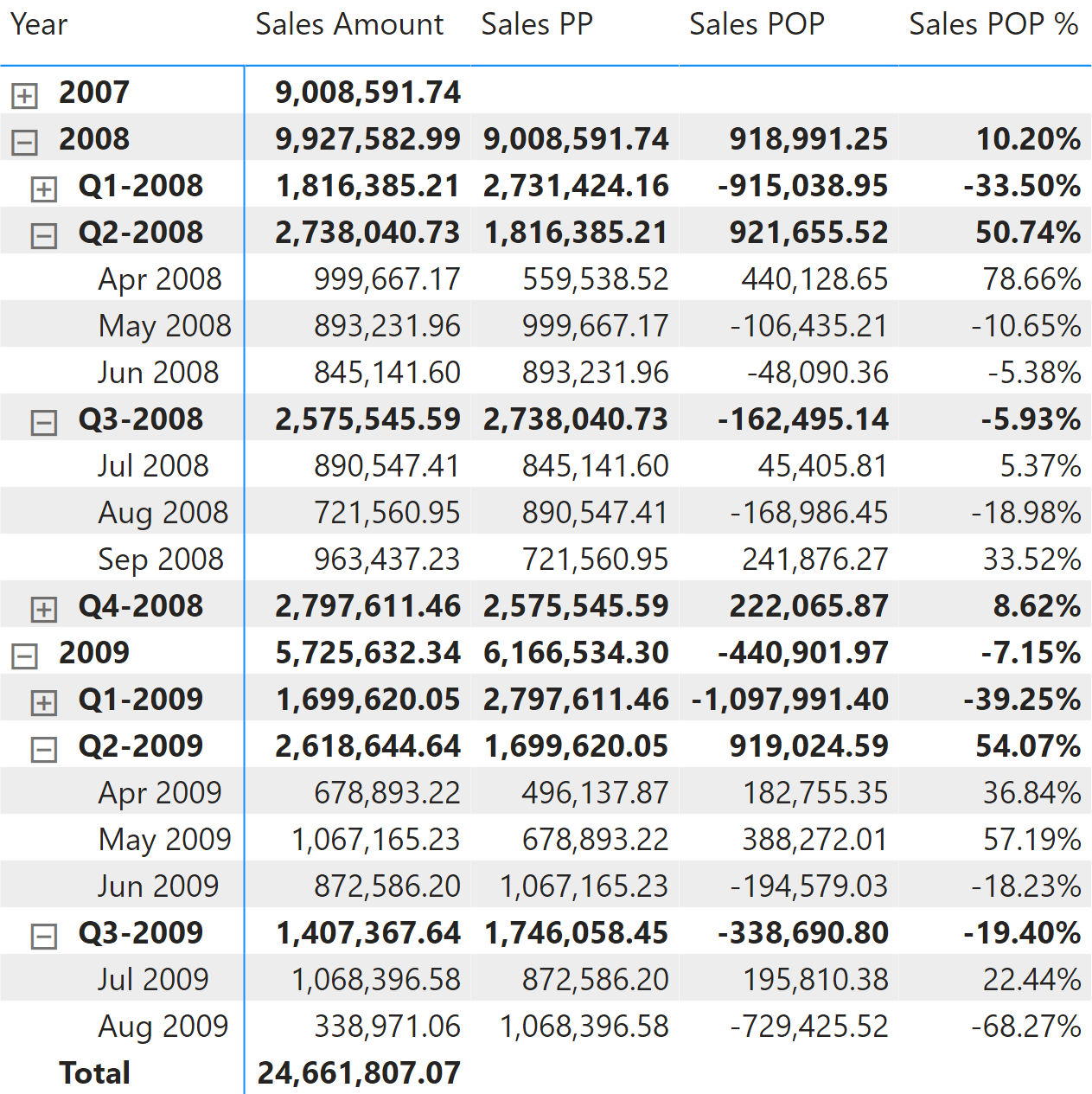
The three measures Sales PP, Sales POP, and Sales POP % redirect the evaluation to the corresponding year, quarter, and month measures depending on the level selected in the report. The ISINSCOPE function detects the level used in the report. The arguments passed to ISINSCOPE are the attributes used in the rows of the Matrix visual from Figure 6. The measures are defined as follows:
Sales POP % :=
SWITCH (
    TRUE,
    ISINSCOPE ( 'Date'[Year Month] ), [Sales MOM %],
    ISINSCOPE ( 'Date'[Year Quarter] ), [Sales QOQ %],
    ISINSCOPE ( 'Date'[Year] ), [Sales YOY %]
)
Sales POP :=
SWITCH (
    TRUE,
    ISINSCOPE ( 'Date'[Year Month] ), [Sales MOM],
    ISINSCOPE ( 'Date'[Year Quarter] ), [Sales QOQ],
    ISINSCOPE ( 'Date'[Year] ), [Sales YOY]
)
Sales PP :=
SWITCH (
    TRUE,
    ISINSCOPE ( 'Date'[Year Month] ), [Sales PM],
    ISINSCOPE ( 'Date'[Year Quarter] ), [Sales PQ],
    ISINSCOPE ( 'Date'[Year] ), [Sales PY]
)
Computing period-to-date growth
The growth of a “to-date” measure is the comparison of said “to-date” measure with the same measure over an equivalent time period with a specific offset. For example, you can compare a year-to-date aggregation against the year-to-date in the previous year, that is with an offset of one year.
All the measures in this set of calculations take care of partial periods. Because data is available only until August 2009 in our example, the measures make sure the previous year does not report dates after August 2008.
Year-over-year-to-date growth
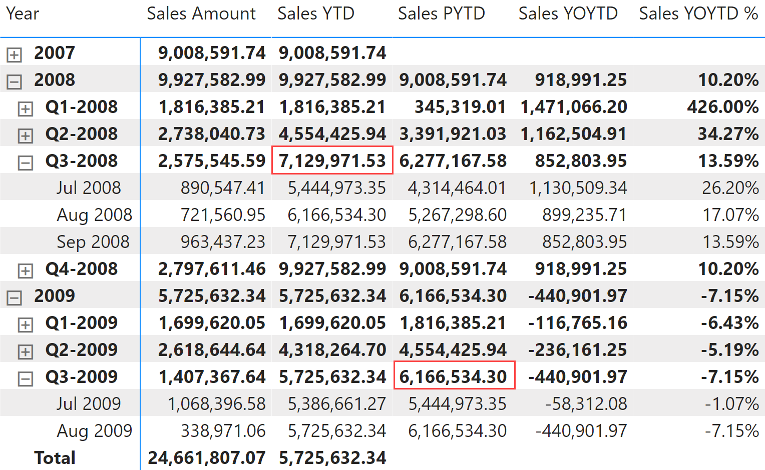
Year-over-year-to-date growth compares the year-to-date at a specific date with the year-to-date in an equivalent month in the previous year. Figure 7 shows that Sales PYTD in 2009 is taking into account transactions only until August 2008. For this reason, Sales YTD of Q3-2008 is 7,129,971.53, whereas Sales PYTD for Q3-2009 is less: 6,166,534.30.
Sales PYTD filters the previous value in Year and all the months in the year less than or equal to the last month visible in the filter context:
Sales PYTD :=
VAR LastMonthInYearAvailable = MAX ( 'Date'[Month Number] )
VAR LastYearAvailable = SELECTEDVALUE ( 'Date'[Year] )
VAR PreviousYearAvailable = LastYearAvailable - 1
VAR Result =
    CALCULATE (
        [Sales Amount],
        REMOVEFILTERS ( 'Date' ),
        'Date'[Month Number] <= LastMonthInYearAvailable,
        'Date'[Year] = PreviousYearAvailable
    )
RETURN
    Result
Sales YOYTD and Sales YOYTD % rely on Sales PYTD to provide their result:
Sales YOYTD :=
VAR ValueCurrentPeriod = [Sales YTD]
VAR ValuePreviousPeriod = [Sales PYTD]
VAR Result =
    IF (
        NOT ISBLANK ( ValueCurrentPeriod ) && NOT ISBLANK ( ValuePreviousPeriod ),
        ValueCurrentPeriod - ValuePreviousPeriod
    )
RETURN
    Result
Sales YOYTD % :=
DIVIDE (
    [Sales YOYTD],
    [Sales PYTD]
)
Quarter-over-quarter-to-date growth
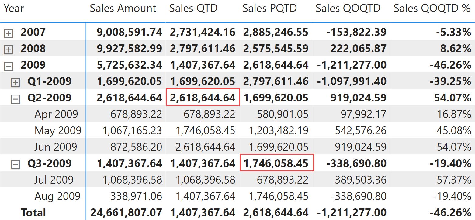
Quarter-over-quarter-to-date growth compares the quarter-to-date at a specific date with the quarter-to-date at an equivalent month in the previous quarter. Figure 8 shows that Sales PQTD in 2009 is taking into account transactions only until May 2009, which is the second month in the quarter. For this reason, Sales QTD of Q2-2009 is 2,618,644.64, whereas Sales PQTD for Q3-2009 is less: 1,746,058.45.
Sales PQTD filters the previous value in Year Quarter Number, and through Month In Quarter Number filters all the months in the quarter less than or equal to the last relative month of the quarter visible in the filter context:
Sales PQTD :=
VAR LastMonthInQuarterAvailable = MAX ( 'Date'[Month In Quarter Number] )
VAR LastYearQuarterAvailable = MAX ( 'Date'[Year Quarter Number] )
VAR PreviousYearQuarterAvailable = LastYearQuarterAvailable - 1
VAR Result =
    CALCULATE (
        [Sales Amount],
        REMOVEFILTERS ( 'Date' ),
        'Date'[Month In Quarter Number] <= LastMonthInQuarterAvailable,
        'Date'[Year Quarter Number] = PreviousYearQuarterAvailable
    )
RETURN
    Result
Sales QOQTD and Sales QOQTD % rely on Sales PQTD to guarantee a fair comparison:
Sales QOQTD :=
VAR ValueCurrentPeriod = [Sales QTD]
VAR ValuePreviousPeriod = [Sales PQTD]
VAR Result =
    IF (
        NOT ISBLANK ( ValueCurrentPeriod ) && NOT ISBLANK ( ValuePreviousPeriod ),
        ValueCurrentPeriod - ValuePreviousPeriod
    )
RETURN
    Result
Sales QOQTD % :=
DIVIDE (
    [Sales QOQTD],
    [Sales PQTD]
)
Comparing period-to-date with a previous full period
Comparing a to-date aggregation with the previous full period is useful when you consider the previous period as a benchmark. Once the current year-to-date reaches 100% of the full previous year, this means we have reached the performance of the previous full period – hopefully in fewer days.
Year-to-date over the full previous year
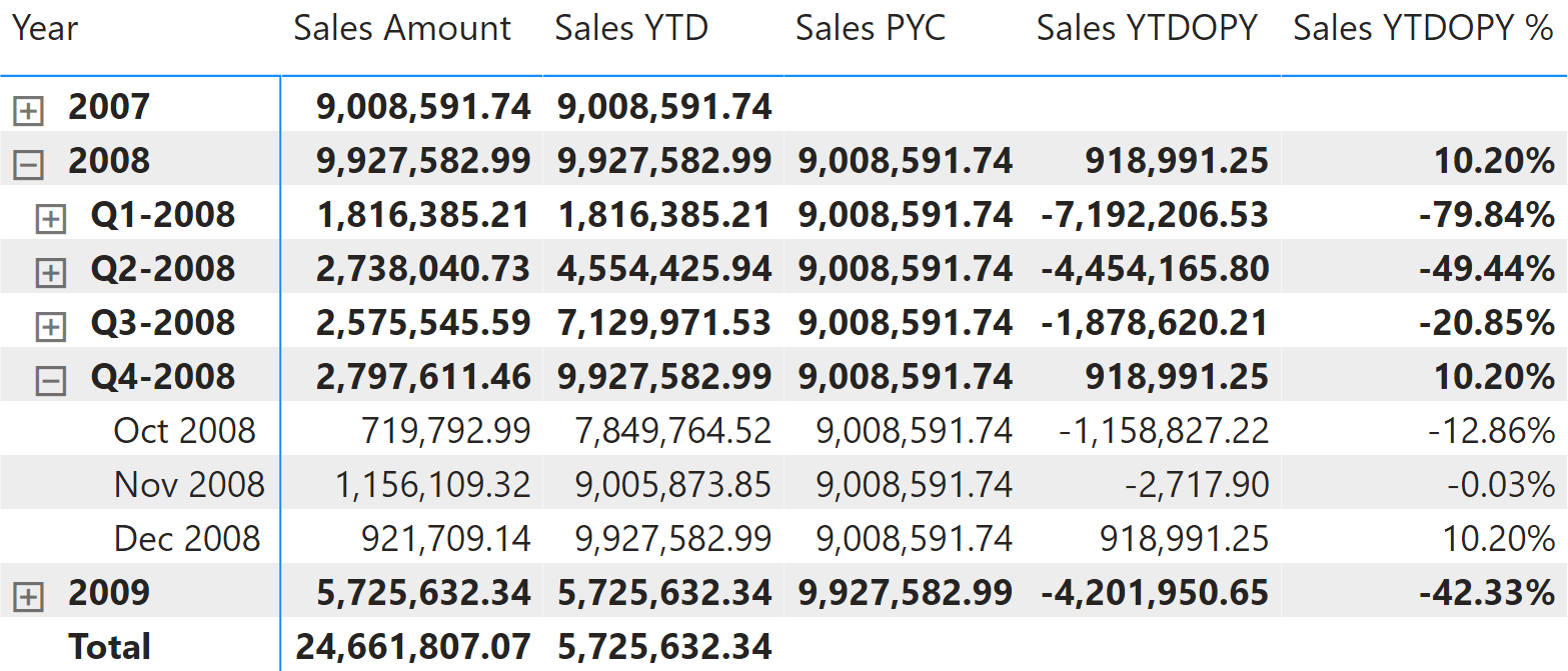
As the name indicates, the year-to-date over the full previous year compares the year-to-date against the entire previous year. Figure 9 shows that in November 2008 (which is close to the end of the year 2008) Sales YTD almost reached the value of Sales Amount for the entire year 2007. Sales YTDOPY % provides an immediate comparison of the year-to-date with the total of the previous year; it shows growth over the previous year when the percentage is positive, which is the case in December 2008.
The year-to-date-over-previous-year growth is computed by using the Sales YTDOPY and Sales YTDOPY % measures; these in turn rely on the Sales YTD measure to compute the year-to-date value, and on the Sales PYC measure to get the sales amount of the entire previous year:
Sales PYC :=
VAR CurrentYearNumber = SELECTEDVALUE ( 'Date'[Year] )
VAR PreviousYearNumber = CurrentYearNumber - 1
VAR Result =
    CALCULATE (
        [Sales Amount],
        REMOVEFILTERS ( 'Date' ),
        'Date'[Year] = PreviousYearNumber
    )
RETURN
    Result
Sales YTDOPY :=
VAR ValueCurrentPeriod = [Sales YTD]
VAR ValuePreviousPeriod = [Sales PYC]
VAR Result =
    IF (
        NOT ISBLANK ( ValueCurrentPeriod ) && NOT ISBLANK ( ValuePreviousPeriod ),
        ValueCurrentPeriod - ValuePreviousPeriod
    )
RETURN
    Result
Sales YTDOPY % :=
DIVIDE (
    [Sales YTDOPY],
    [Sales PYC]
)
Quarter-to-date over full previous quarter
As the name indicates, the quarter-to-date over the full previous quarter compares the quarter-to-date against the entire previous quarter. Figure 10 shows that in May 2009, Sales QTD exceeded the value of Sales Amount for the entire previous quarter (Q1-2009). Sales QTDOPQ% provides an immediate comparison of the quarter-to-date with the total of the previous quarter; it shows growth over the previous quarter when the percentage is positive, which is the case in May and June 2009.
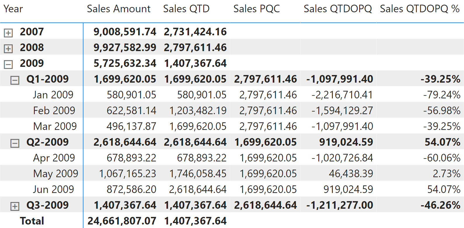
The quarter-to-date-over-previous-quarter growth is computed by using the Sales QTDOPQ and Sales QTDOPQ % measures; these in turn rely on the Sales QTD measure to compute the quarter-to-date value and on the Sales PQC measure to get the sales amount of the entire previous quarter:
Sales PQC :=
VAR CurrentYearQuarterNumber = SELECTEDVALUE ( 'Date'[Year Quarter Number] )
VAR PreviousYearQuarterNumber = CurrentYearQuarterNumber - 1
VAR Result =
    CALCULATE (
        [Sales Amount],
        REMOVEFILTERS ( 'Date' ),
        'Date'[Year Quarter Number] = PreviousYearQuarterNumber
    )
RETURN
    Result
Sales QTDOPQ :=
VAR ValueCurrentPeriod = [Sales QTD]
VAR ValuePreviousPeriod = [Sales PQC]
VAR Result =
    IF (
        NOT ISBLANK ( ValueCurrentPeriod )
            && NOT ISBLANK ( ValuePreviousPeriod ),
        ValueCurrentPeriod - ValuePreviousPeriod
    )
RETURN
    Result
Sales QTDOPQ % :=
DIVIDE (
    [Sales QTDOPQ],
    [Sales PQC]
)
Using moving annual total calculations
A common way to aggregate data over several months is by using the moving annual total instead of the year-to-date. The moving annual total includes the last 12 months of data. For example, the moving annual total for March 2009 includes data from April 2008 to March 2009.
Moving annual total
Sales MAT computes the moving annual total, as shown in Figure 11.
The Sales MAT measure defines a range over the Year Month Number column that includes the months of one complete year from the last month in the filter context:
Sales MAT :=
VAR MonthsInRange = 12
VAR LastMonthRange = MAX ( 'Date'[Year Month Number] )
VAR FirstMonthRange = LastMonthRange - MonthsInRange + 1
VAR Result =
    CALCULATE (
        [Sales Amount],
        REMOVEFILTERS ( 'Date' ),
        'Date'[Year Month Number] >= FirstMonthRange
            && 'Date'[Year Month Number] <= LastMonthRange
    )
RETURN
    Result
Moving annual total growth
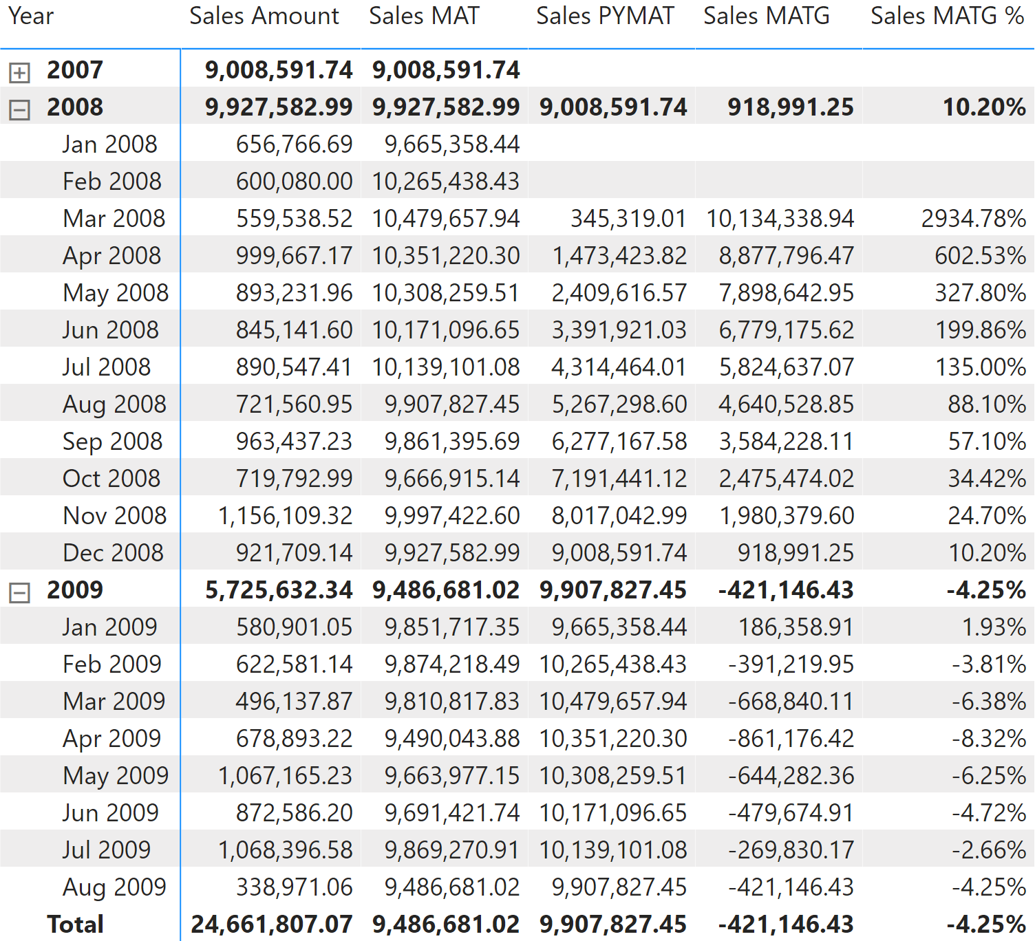
The moving annual total growth is computed by using the Sales PYMAT, Sales MATG, and Sales MATG % measures, which in turn rely on the Sales MAT measure. The Sales MAT measure starts to provide accurate values one year after the first sale ever – once it has been able to collect one full year of data – and it is not protected in case the current time period is shorter than a full year.
For example, the amount for the year 2009 of Sales PYMAT is 9,927,582.99, which corresponds to the Sales Amount of the entire year 2008 as shown in Figure 11 (see previous section). When compared with sales in 2009, this produces a comparison of 8 months – data being only available until August 2009 – with the whole year 2008. Similarly, you can see that Sales MATG % starts in March 2008 with very high values and stabilizes after a year. This behavior is by design: the moving annual total is usually computed at the month granularity to show trends in a chart.
The measures are defined as follows:
Sales PYMAT :=
VAR MonthsInRange = 12
VAR LastMonthRange =
    MAX ( 'Date'[Year Month Number] ) - MonthsInRange
VAR FirstMonthRange =
    LastMonthRange - MonthsInRange + 1
VAR Result =
    CALCULATE (
        [Sales Amount],
        REMOVEFILTERS ( 'Date' ),
        'Date'[Year Month Number] >= FirstMonthRange
            && 'Date'[Year Month Number] <= LastMonthRange
    )
RETURN
    Result
Sales MATG :=
VAR ValueCurrentPeriod = [Sales MAT]
VAR ValuePreviousPeriod = [Sales PYMAT]
VAR Result =
    IF (
        NOT ISBLANK ( ValueCurrentPeriod )
            && NOT ISBLANK ( ValuePreviousPeriod ),
        ValueCurrentPeriod - ValuePreviousPeriod
    )
RETURN
    Result
Sales MATG % :=
DIVIDE (
    [Sales MATG],
    [Sales PYMAT]
)
Moving averages
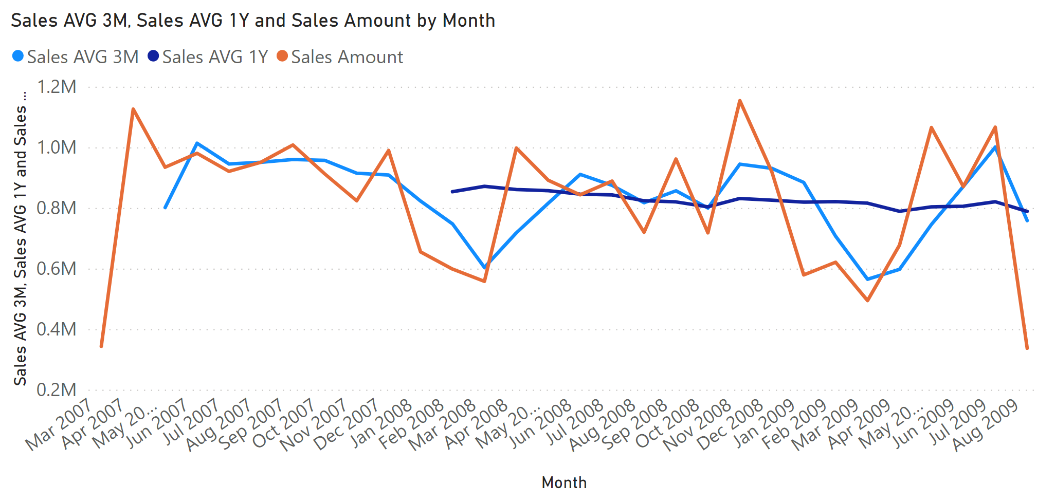
The moving average is typically used to display trends in line charts. Figure 12 includes the moving average of three months (Sales AVG 3M) and a year (Sales AVG 1Y).
Moving average 3 months
The Sales AVG 3M measure computes the moving average over three months by iterating the last three months obtained in the Period3M variable:
Sales AVG 3M :=
VAR MonthsInRange = 3
VAR LastMonthRange =
    MAX ( 'Date'[Year Month Number] )
VAR FirstMonthRange =
    LastMonthRange - MonthsInRange + 1
VAR Period3M =
    FILTER (
        ALL ( 'Date'[Year Month Number] ),
        'Date'[Year Month Number] >= FirstMonthRange
            && 'Date'[Year Month Number] <= LastMonthRange
    )
VAR Result =
    IF (
        COUNTROWS ( Period3M ) >= MonthsInRange,
        CALCULATE (
            AVERAGEX ( Period3M, [Sales Amount] ),
            REMOVEFILTERS ( 'Date' )
        )
    )
RETURN
    Result
Moving average 1 year
The Sales AVG 1Y measure computes the moving average over one year by iterating the last 12 months stored in the Period1Y variable:
Sales AVG 1Y :=
VAR MonthsInRange = 12
VAR LastMonthRange =
    MAX ( 'Date'[Year Month Number] )
VAR FirstMonthRange =
    LastMonthRange - MonthsInRange + 1
VAR Period1Y =
    FILTER (
        ALL ( 'Date'[Year Month Number] ),
        'Date'[Year Month Number] >= FirstMonthRange
            && 'Date'[Year Month Number] <= LastMonthRange
    )
VAR Result =
    IF (
        COUNTROWS ( Period1Y ) >= MonthsInRange,
        CALCULATE (
            AVERAGEX ( Period1Y, [Sales Amount] ),
            REMOVEFILTERS ( 'Date' )
        )
    )
RETURN
    Result
Managing years with more than 12 months
As we stated in the introduction, this pattern works even in scenarios where one year contains more than 12 months. For example, accounting oftentimes requires a 13th month containing the year-end adjustments. In these scenarios, it is important to set the values in the Date table correctly. Specifically, the Year Month Number column must store a sequential number for each month of the year; therefore, the same month in the previous year can be obtained by just subtracting 13 from the value of the current month if the year contains 13 months.
Moreover, you need to pay attention to the content of the Month and Year Month columns. Indeed, these columns must contain a proper name for the 13th month, and that choice depends on how you plan to show the month in both the fiscal and Gregorian calendars.
If the report shows only the fiscal year, you can choose any name and you will always show 13 months. If you need to show both fiscal and Gregorian calendar hierarchies, then you should decide between the following options: you can show the 13th month as a separate month in the Gregorian calendar; or you can decide to merge it under the corresponding Gregorian month, which means you are still showing 12 months when displaying the Gregorian calendar.
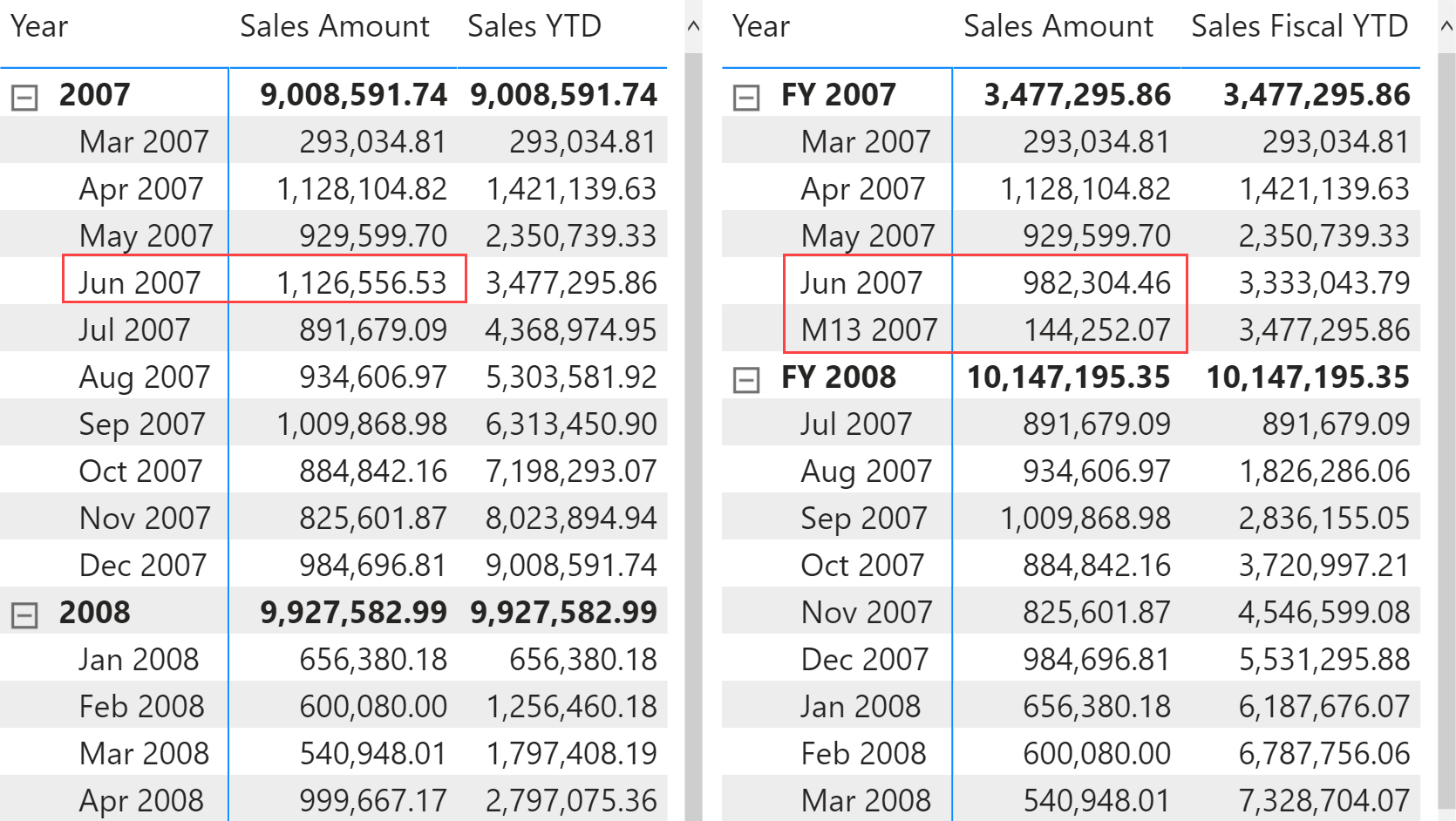
For example, Figure 13 shows the 13th month named “M13”. Its position is right after June, because the fiscal calendar ends in June. The month is visible both in the fiscal and in the Gregorian calendars.
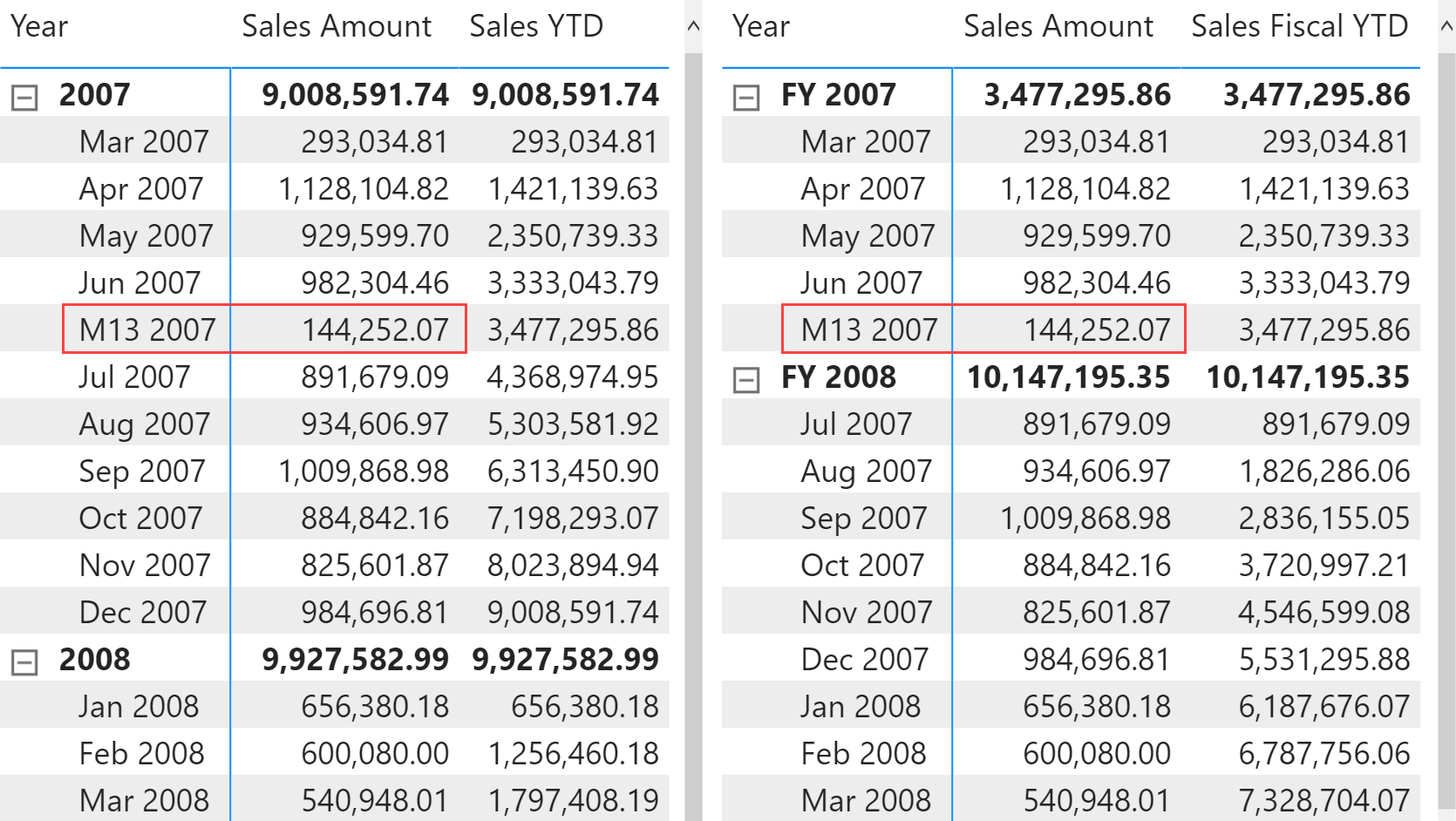
Figure 14 shows the result of a different choice, where the 13th month is visible only in the fiscal calendar. When the report is being browsed by the Gregorian calendar, the value of the 13th month is merged with that of June. Therefore, the Gregorian calendar is still showing 12 months.
If you want to merge June with the 13th month as shown on the left side of Figure 14, then you must assign the proper values to the columns in the Date table; it is then no longer possible to share the same columns for both fiscal and Gregorian calendars. The columns for the fiscal calendar must differentiate between the 12th and 13th months, whereas the columns for the Gregorian calendar will share the values for the month name and number. Therefore, the Date table still contains 13 months, but two of them share the same values in the Gregorian set of columns. By doing so, the report merges rows with the same value in the months columns and the user obtains the desired result.
You can find the set of values for the figures shown in this section in the demo files ”Month-related calculations – 13 Fiscal and 13 Calendar Months.pbix” and ”Month-related calculations – 13 Fiscal and 12 Calendar Months.pbix”, respectively, where the Year Month, Year Month Number, Month, and Month Number columns for the Gregorian calendar have corresponding Fiscal Year Month, Fiscal Year Month Number, Fiscal Month, and Fiscal Month Number columns for the fiscal calendar.
Clear filters from the specified tables or columns.
REMOVEFILTERS ( [<TableNameOrColumnName>] [, <ColumnName> [, <ColumnName> [, … ] ] ] )
The second table expression will be evaluated for each row in the first table. Returns the crossjoin of the first table with these results.
GENERATE ( <Table1>, <Table2> )
When a column name is given, returns a single-column table of unique values. When a table name is given, returns a table with the same columns and all the rows of the table (including duplicates) with the additional blank row caused by an invalid relationship if present.
VALUES ( <TableNameOrColumnName> )
Returns true when the specified column is the level in a hierarchy of levels.
ISINSCOPE ( <ColumnName> )
This pattern is included in the book DAX Patterns, Second Edition.


Video

Do you prefer a video?
This pattern is also available in video format. Take a peek at the preview, then unlock access to the full-length video on SQLBI.com.Watch the full video — 71 min.
Downloads
Download the sample files for Power BI / Excel 2016-2019: