Filtering An Excel Cube Function Report By A List Of Manually-Entered Values

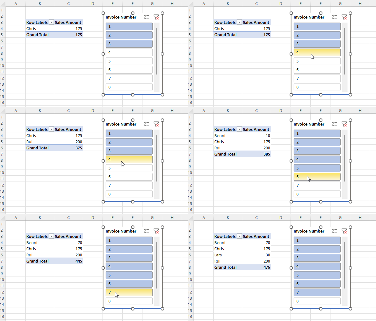
In Power BI there’s a popular custom visual called “Filter by list” that lets you filter a Power BI report by any list of values that you paste into it. It can save you a lot of time in some scenarios, for example if you need to copy a list of values from another application and select those values in a slicer. In this post I’ll show how to recreate the same functionality in an Excel report connected to Power BI, Analysis Services or the Excel Data Model/Power Pivot using cube functions and dynamic arrays.

To show how I’m going to use a super-simple model built using Power Pivot consisting of the following single table:

The only other thing to note about the model is that it contains a measure called Sales Amount that sums up the values in the Sales column:

Sales Amount:=SUM(Sales[Sales])

Here’s what a PivotTable connected to this model looks like:

The aim here is to recreate this PivotTable using cube functions and allow the user to enter the list of invoice numbers used to slice the data either manually or by copy-and-pasting them into a table.

The first step is to create an Excel table (which I’ve called InvoiceNumbers) to hold the invoice numbers the user enters:

The next thing to do is to generate the text of the MDX set expression representing the list of invoice numbers in this table, which I’ve put in cell D2:

="{" & TEXTJOIN(",",TRUE, "[Sales].[Invoice Number].[Invoice Number].&[" & InvoiceNumbers & "]" ) &"}"

This text is used to create two named sets using the CUBESET function. The first, which I’ve put in cell D3, simply returns the set of invoice numbers that you get from evaluating the above MDX expression:

=CUBESET("ThisWorkbookDataModel", $D$2, "Invoice Numbers")

The second named set, in D4, is more complicated: it returns the set of customers that have sales for these invoice numbers.

=CUBESET(
"ThisWorkbookDataModel", 
"NONEMPTY( [Sales].[Customer].[Customer].MEMBERS, {[Measures].[Sales Amount]} * " & $D$2 & ")",
"Customers")

Last of all are the cube functions that display the report itself. In cell E6 is the CUBEVALUE function returning the measure Sales Amount:

=CUBEMEMBER("ThisWorkbookDataModel", "[Measures].[Sales Amount]")

In D7 is the formula (using the technique I blogged about here) to get the list of Customers returned by the second named set above:

=MAKEARRAY(
CUBESETCOUNT($D$4), 
1, 
LAMBDA(r,c, CUBERANKEDMEMBER("ThisWorkbookDataModel", $D$4, r))
)

Finally, in D8, is the expression that gets the Sales Amount values for each customer, sliced also by the set of selected invoice numbers:

=MAKEARRAY(
CUBESETCOUNT($D$4),
1,
LAMBDA(r,c,
CUBEVALUE("ThisWorkbookDataModel", INDEX($D$7#,r), $D$3, $E$6))
)

Here are the formulas all together:

And here it all is working:

One last point: to keep things simple I’ve not included any error handling, which means that if a user enters a blank value or a value that isn’t an invoice number in the table the whole thing will break. To handle errors using the technique I blogged about here, alter the formula in D2 to:

="{"&
TEXTJOIN(
",",
TRUE,
LET(
MemberExpression,
"[Sales].[Invoice Number].[Invoice Number].&["&InvoiceNumbers&"]",
"IIF(ISERROR(STRTOMEMBER("""&MemberExpression&""")), {}, STRTOMEMBER("""&MemberExpression&"""))")
) &"}"

You can download the example workbook here (although it may not work unless you’ve got a version of Excel with dynamic arrays enabled).