

By introducing Azure Synapse Analytics in late 2019, Microsoft created a whole new perspective when it comes to data treatment. Some core concepts, such as traditional data warehousing, came under more scrutiny, while various fresh approaches started to pop up after data nerds became aware of the new capabilities that Synapse brought to the table.
Not that Synapse made a strong impact on data ingestion, transformation, and storage options only – it also offered a whole new set of possibilities for data serving and visualization!
Therefore, in this series of blog posts, I will try to explore how Power BI works in synergy with the new platform. What options we, Power BI developers, have when working with Synapse? In which data analytics scenarios, Synapse will play on the edge, helping you to achieve the (im)possible? When would you want to take advantage of the innovative solutions within Synapse, and when would you be better sticking with more conventional approaches? What are the best practices when using Power BI – Synapse combo, and which parameters should you evaluate before making a final decision on which path to take.
Once we’re done, I believe that you should get a better understanding of the “pros” and “cons” for each of the available options when it comes to integration between Power BI and Synapse.
Special thanks to Jovan Popovic and Filip Popovic from Microsoft, who helped me understand key concepts and architecture of Synapse
- Power BI & Synapse Part 1 – The Art of (im)possible!
- Power BI & Synapse Part 2 – What Synapse brings to Power BI table?
- Power BI & Synapse Part 3 – Keep the Tradition!
Don’t get me wrong – the theory is nice, and you should definitely spend your time trying to absorb basic architectural concepts of new technology, tool, or feature. Because, if you don’t understand how something works under the hood, there is a great chance that you won’t take maximum advantage of it.
But, putting this theoretical knowledge on a practice test is what makes the most interesting part! At least for me:)…It reminds me of the car production process: they build everything, you read the specs and you are impressed! Features, equipment…However, it’s all irrelevant until they put the car on a crash test and get a proper reality check.
Therefore, this article will be like a crash test for the Serverless SQL pool within Synapse Analytics – lot of different scenarios, tests, demos, measures, etc.
Serverless SQL pool – The next big thing
I’ve already written about the Serverless SQL pool, and I firmly believe that it is the next big thing when it comes to dealing with large volumes of semi-structured or non-structured data.
The greatest advantage of the Serverless SQL pool is that you can query the data directly from the CSV, parquet, or JSON files, stored in your Azure Data Lake, without the need to transfer the data! Even more, you can write plain T-SQL to retrieve the data directly from the files! But, let’s see how this works in reality in various use-cases, and, the most important thing, how much each of the solutions will cost you!

There are still some things that Microsoft won’t charge you for data processing when using Synapse Serverless SQL pool, such as:
- Server-level metadata (logins, roles, and server-level credentials)
- Databases you create in your endpoint. Those databases contain only metadata (users, roles, schemas, views, inline table-valued functions, stored procedures, external data sources, external file formats, and external tables)
- DDL statements, except for the CREATE STATISTICS statement because it processes data from storage based on the specified sample percentage
- Metadata-only queries
Scenario
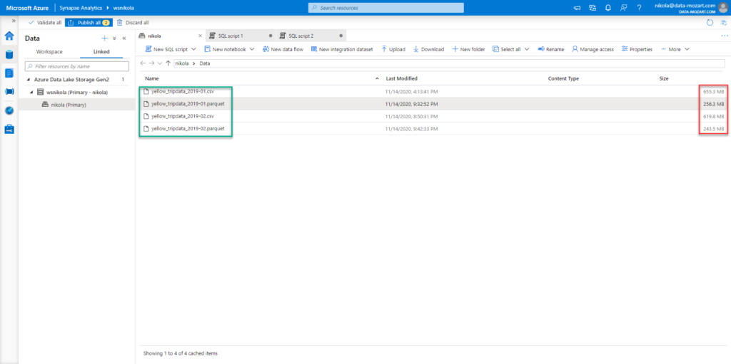
Here is the scenario: I have two CSV files related to the NYC taxi dataset, that I’ve already used in one of the previous demos. One contains data about all yellow cab rides from January 2019 (650 MB), while the other contains data from February 2019 (620 MB).
I’ve created two separate views, for each month’s data. The idea is to check what happens when we query the data from Power BI under multiple different conditions.
Here is the T-SQL for creating a view over a single month:
DROP VIEW IF EXISTS taxi201902csv;
GO

CREATE VIEW taxi201902csv AS
SELECT
	VendorID
	,cast(tpep_pickup_datetime as DATE) tpep_pickup_datetime
	,cast(tpep_dropoff_datetime as DATE) tpep_dropoff_datetime
	,passenger_count
	,trip_distance
	,RateCodeID
	,store_and_fwd_flag
	,PULocationID
	,DOLocationID
	,payment_type
	,fare_amount
	,extra
	,mta_tax
	,tip_amount
	,tolls_amount
	,improvement_surcharge
	,total_amount
	,congestion_surcharge
FROM
    OPENROWSET(
        BULK N'https://nikola.dfs.core.windows.net/nikola/Data/yellow_tripdata_2019-02.csv',
        FORMAT = 'CSV',
        PARSER_VERSION='2.0',
        HEADER_ROW = TRUE
    )
	WITH(
		VendorID INT,
		tpep_pickup_datetime DATETIME2,
		tpep_dropoff_datetime DATETIME2,
		passenger_count INT,
		trip_distance DECIMAL(10,2),
		RateCodeID INT,
		store_and_fwd_flag VARCHAR(10),
		PULocationID INT,
		DOLocationID INT,
		payment_type INT,
		fare_amount DECIMAL(10,2),
		extra DECIMAL(10,2),
		mta_tax DECIMAL(10,2),
		tip_amount DECIMAL(10,2),
		tolls_amount DECIMAL(10,2),
		improvement_surcharge DECIMAL(10,2),
		total_amount DECIMAL(10,2),
		congestion_surcharge DECIMAL(10,2)
	)
    AS [taxi201902csv]
I am using WITH block to explicitly define data types, as if you don’t do it, all your character columns will be automatically set to VARCHAR(8000), and consequentially more memory expensive.
As you can notice, I’ve renamed my generic column names from CSV files, so they now look more readable. I’ve also cast DateTime columns to Date type only, as I don’t need the time portion for this demo. This way, we’ve reduced the cardinality and the whole data model size consequentially. Let’s check how many records each of these files contains:
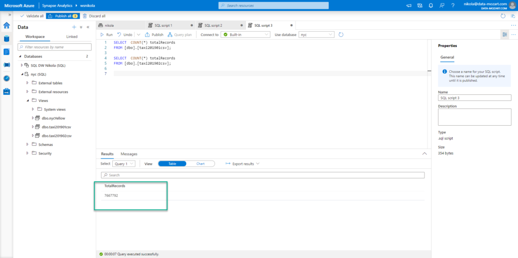
January contains ~7.6 million records, while February has ~7 million records.
Additionally, I’ve also applied the same logic and built two views over exactly the same portion of data coming from parquet files. So, we can compare metrics between CSV and Parquet files.
Views used for views over Parquet files were built slightly different, using FILENAME() and FILEPATH() functions to eliminate unnecessary partitions:
DROP VIEW IF EXISTS taxi201901parquet;
GO

CREATE VIEW taxi201901parquet AS
SELECT
        VendorID
        ,CAST(TpepPickupDatetime AS DATE) TpepPickupDatetime
        ,CAST(TpepDropoffDatetime AS DATE) TpepDropoffDatetime
        ,PassengerCount
        ,TripDistance
        ,PuLocationId
        ,DoLocationId
        ,StartLon
        ,StartLat
        ,EndLon
        ,EndLat
        ,RateCodeId
        ,StoreAndFwdFlag
        ,PaymentType
        ,FareAmount
        ,Extra
        ,MtaTax
        ,ImprovementSurcharge
        ,TipAmount
        ,TollsAmount
        ,TotalAmount
FROM
    OPENROWSET(
        BULK 'puYear=*/puMonth=*/*.snappy.parquet',
        DATA_SOURCE = 'YellowTaxi',
        FORMAT='PARQUET'
    ) nyc
WHERE
    nyc.filepath(1) = 2019
    AND nyc.filepath(2) IN (1)
    AND tpepPickupDateTime BETWEEN CAST('1/1/2019' AS datetime) AND CAST('1/31/2019' AS datetime)
As specified in the best practices for using Serverless SQL pool in Synapse, we explicitly instructed our query to target only year 2019 and only month of January! This will reduce the amount of data for scanning and processing. We didn’t have to do this for our CSV files, as they were already partitioned per month and saved like that.
One important disclaimer: As the usage of the Serverless SQL pool is being charged per volume of the data processed (it’s currently priced starting at 5$/TB of processed data), I will not measure performance in terms of speed. I want to focus solely on the analysis of data volume processed and costs generated by examining different scenarios.
CSV vs Parquet – What do I need to know?
Before we proceed with testing, a little more theory…As I plan to compare data processing between CSV and Parquet files, I believe we should understand the key differences between these two types:
- In Parquet files, data is compressed in a more optimal way. As you may recall from one of the screenshots above, a parquet file consumes approximately 1/3 of memory compared to a CSV file that contains the same portion of data
- Parquet files support column storage format – that being said, columns within Parquet file are physically separated, which means that you don’t need to scan the whole file if you need data from few columns only! On the opposite, when you’re querying a CSV file, every time you send the query, it will scan the whole file, even if you need data from one single column
- For those coming from the traditional SQL world, you can think of CSV vs Parquet, such as row-store vs columnar databases
Use Case #1 – Import CSV data into Power BI
Let’s start with the most obvious and desirable scenario – using Import mode to ingest all the data into Power BI, and performing data refresh to check how much it will cost us.
One last thing before we get our hands dirty – in Synapse Analytics, there is still not a feature to measure the cost of a specific query. You can check the volume of processed data on a daily, weekly, or monthly level. Additionally, you can set the limits if you want, on each of those time-granularity levels – more on that in this article.
This feature is also relatively new, so I’m glad to see that Synapse permanently makes progress in a promising way of providing full cost transparency.
Since we can’t measure exact cost of every single query, I will try to calculate the figures by querying DMV within master database, using the following T-SQL:
SELECT * FROM sys.dm_external_data_processed
WHERE type = 'daily'
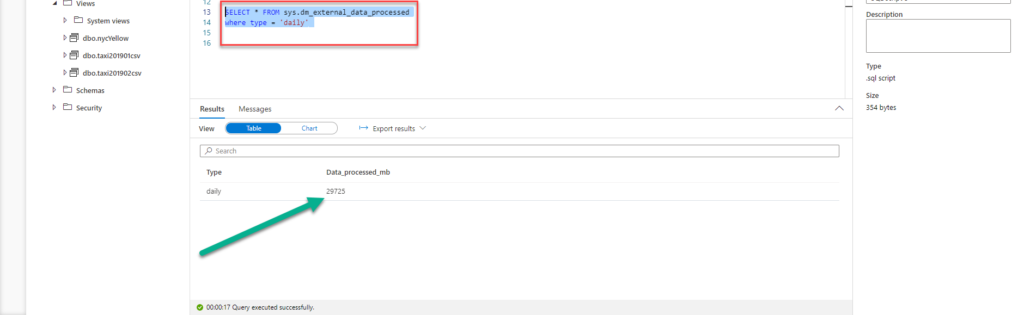
So, my starting point for today is around 29.7 GB, and I will calculate the difference each time I target the Serverless SQL pool to get the data.
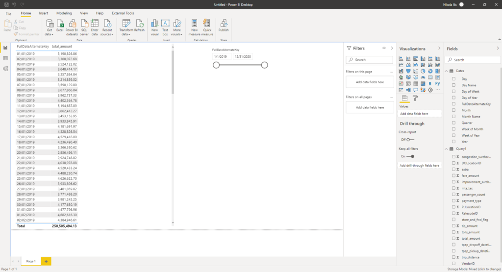
Ok, going back to the first scenario, I will import the data into Power BI, for both months from CSV files:
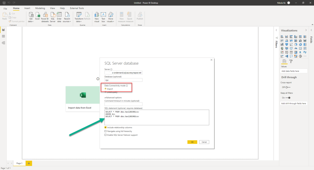
The most fascinating thing is that I’m writing plain T-SQL, so my users don’t even know that they are getting the data directly from CSV files! I’m using UNION ALL, as I’m sure that there are no identical records in my two views, and in theory, it should run faster than UNION, but I’ve could also create a separate view using this same T-SQL statement, and then use that joint view in Power BI.
I will need a proper date dimension table for testing different scenarios, and I will create it using Power Query. This date table will be in Import mode in all scenarios, so it should not affect the amount of processed data from the Serverless SQL pool. Here is the M code for the date table:
let
    StartDate = #date(StartYear,1,1),
    EndDate = #date(EndYear,12,31),
    NumberOfDays = Duration.Days( EndDate - StartDate ),
    Dates = List.Dates(StartDate, NumberOfDays+1, #duration(1,0,0,0)),
    #"Converted to Table" = Table.FromList(Dates, Splitter.SplitByNothing(), null, null, ExtraValues.Error),
    #"Renamed Columns" = Table.RenameColumns(#"Converted to Table",{{"Column1", "FullDateAlternateKey"}}),
    #"Changed Type" = Table.TransformColumnTypes(#"Renamed Columns",{{"FullDateAlternateKey", type date}}),
    #"Inserted Year" = Table.AddColumn(#"Changed Type", "Year", each Date.Year([FullDateAlternateKey]), type number),
    #"Inserted Month" = Table.AddColumn(#"Inserted Year", "Month", each Date.Month([FullDateAlternateKey]), type number),
    #"Inserted Month Name" = Table.AddColumn(#"Inserted Month", "Month Name", each Date.MonthName([FullDateAlternateKey]), type text),
    #"Inserted Quarter" = Table.AddColumn(#"Inserted Month Name", "Quarter", each Date.QuarterOfYear([FullDateAlternateKey]), type number),
    #"Inserted Week of Year" = Table.AddColumn(#"Inserted Quarter", "Week of Year", each Date.WeekOfYear([FullDateAlternateKey]), type number),
    #"Inserted Week of Month" = Table.AddColumn(#"Inserted Week of Year", "Week of Month", each Date.WeekOfMonth([FullDateAlternateKey]), type number),
    #"Inserted Day" = Table.AddColumn(#"Inserted Week of Month", "Day", each Date.Day([FullDateAlternateKey]), type number),
    #"Inserted Day of Week" = Table.AddColumn(#"Inserted Day", "Day of Week", each Date.DayOfWeek([FullDateAlternateKey]), type number),
    #"Inserted Day of Year" = Table.AddColumn(#"Inserted Day of Week", "Day of Year", each Date.DayOfYear([FullDateAlternateKey]), type number),
    #"Inserted Day Name" = Table.AddColumn(#"Inserted Day of Year", "Day Name", each Date.DayOfWeekName([FullDateAlternateKey]), type text)
in
    #"Inserted Day Name"
It took a while to load the data in the Power BI Desktop, so let’s check now some key metrics.
- My table has ~ 14.7 million rows
- My whole data model size is ~92 MB, as the data is optimally compressed within Power BI Desktop (we’ve reduced the cardinality of DateTime columns)

Once I’ve created my table visual, displaying total records per date, my daily data processed volume is ~33.3 GB. Let’s refresh the data model to check how expensive it would be. So, Power BI Desktop will now go to a Serverless SQL pool, querying data from my two views, but don’t forget that in the background are two CSV files as an ultimate source of our data!
After the refresh, my daily value had increased to ~36.9 GB, which means that this refresh costs me ~3.6 GB. In terms of money, that’s around 0.018 $ (0.0036 TB x 5 USD).
In this use case, it would cost me money only when my Power BI model is being refreshed! Simply said, if I refresh my data model once per day, this report will cost me 54 cents per month.
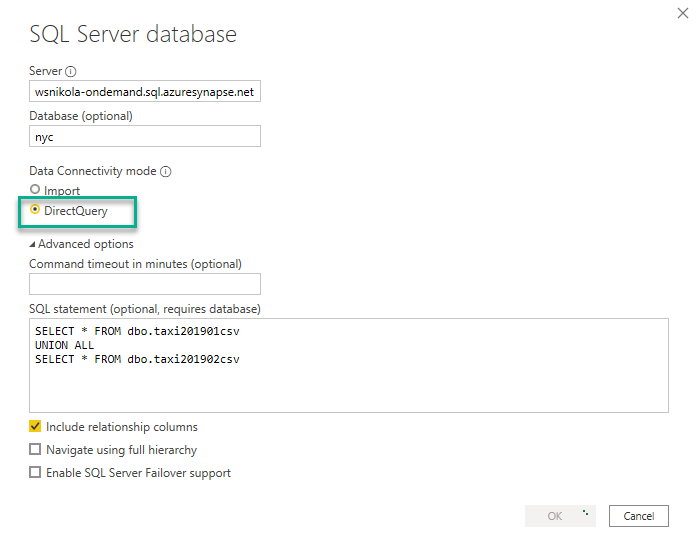
Use Case #2 – DirectQuery over CSV files
Let’s now check what would happen if we use exactly the same query, but instead of importing data into Power BI Desktop, we will use the DirectQuery option.
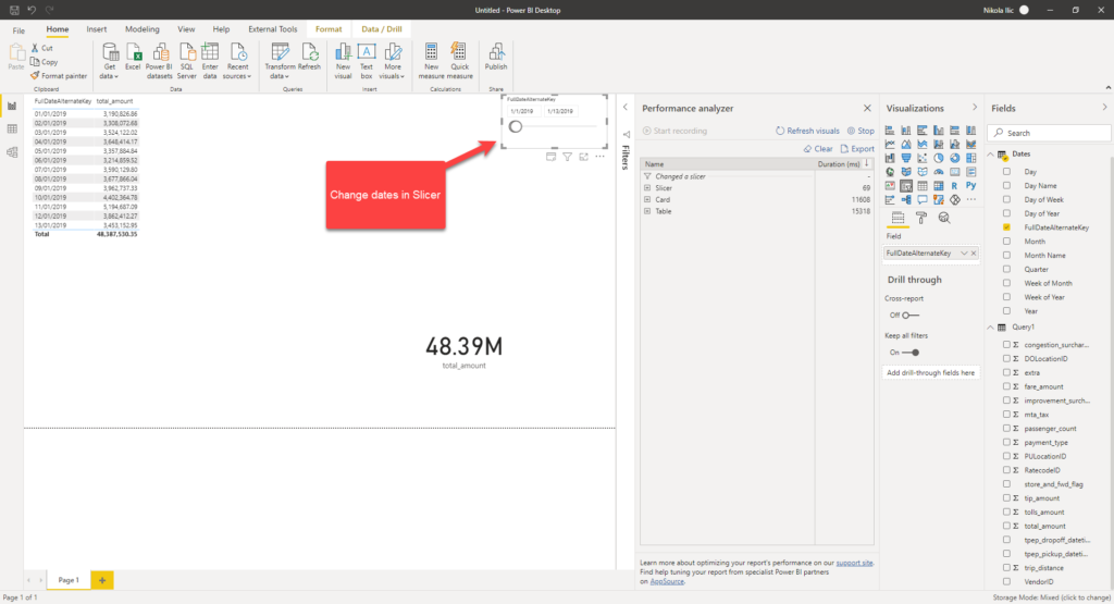
Let’s first interact with the date slicer, so we can check how much this will cost us. My starting point for measuring is ~87.7 GB and this is how my report looks like:
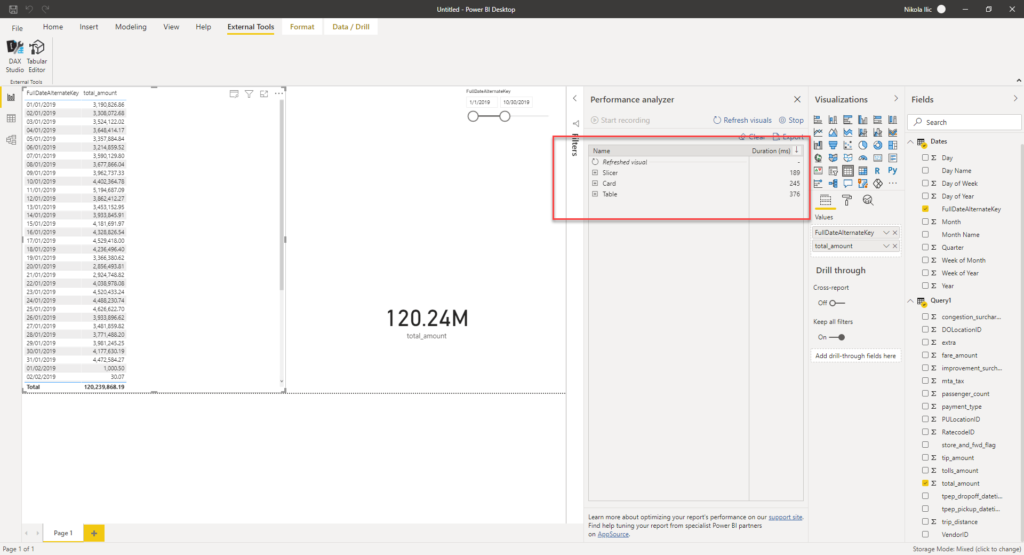
Refreshing the whole query burned out ~2.8 GB, which is ~0.014$. Now, this is for one single visual on the page! Keep in mind that when you’re using DirectQuery, each visual will generate a separate query to the underlying data source. Let’s check what happens when I add another visual on the page:

Now, this query costs me ~4 GB, which is 0.02$. As you can conclude, increasing the number of the visuals on your report canvas, will also increase the costs.
One more important thing to keep in mind: these costs are per user! So, if you have 10 users running this same report in parallel, you should multiply costs by 10, as new query will be generated for each visual and for each user.
Use Case #3 – Use Date slicer in DirectQuery mode
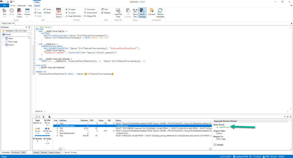
Now, I want to check what happens if I select a specific date range within my slicer, for example between January 1st and January 13th:
The first thing I notice is that query cost me exactly the same! The strange thing is, if I look at the SQL query generated to retrieve the data, I can see the engine was clever enough to apply date filter in the WHERE clause:
/*Query 1*/
SELECT
TOP (1000001) [semijoin1].[c1],SUM([a0])
 AS [a0]
FROM
(
(
SELECT [t1].[tpep_pickup_datetime] AS [c14],[t1].[total_amount] AS [a0]
FROM
(
(SELECT * FROM dbo.taxi201901csv
UNION ALL
SELECT * FROM dbo.taxi201902csv
)
)
 AS [t1]
)
 AS [basetable0]
 INNER JOIN
(
(SELECT 3 AS [c1],CAST( '20190101 00:00:00' AS datetime) AS [c14] )  UNION ALL
(SELECT 4 AS [c1],CAST( '20190102 00:00:00' AS datetime) AS [c14] )  UNION ALL
(SELECT 5 AS [c1],CAST( '20190103 00:00:00' AS datetime) AS [c14] )  UNION ALL
(SELECT 6 AS [c1],CAST( '20190104 00:00:00' AS datetime) AS [c14] )  UNION ALL
(SELECT 7 AS [c1],CAST( '20190105 00:00:00' AS datetime) AS [c14] )  UNION ALL
(SELECT 8 AS [c1],CAST( '20190106 00:00:00' AS datetime) AS [c14] )  UNION ALL
(SELECT 9 AS [c1],CAST( '20190107 00:00:00' AS datetime) AS [c14] )  UNION ALL
(SELECT 10 AS [c1],CAST( '20190108 00:00:00' AS datetime) AS [c14] )  UNION ALL
(SELECT 11 AS [c1],CAST( '20190109 00:00:00' AS datetime) AS [c14] )  UNION ALL
(SELECT 12 AS [c1],CAST( '20190110 00:00:00' AS datetime) AS [c14] )  UNION ALL
(SELECT 13 AS [c1],CAST( '20190111 00:00:00' AS datetime) AS [c14] )  UNION ALL
(SELECT 14 AS [c1],CAST( '20190112 00:00:00' AS datetime) AS [c14] )  UNION ALL
(SELECT 15 AS [c1],CAST( '20190113 00:00:00' AS datetime) AS [c14] )
)
 AS [semijoin1] on
(
([semijoin1].[c14] = [basetable0].[c14])
)
)
GROUP BY [semijoin1].[c1]

/*Query 2*/
SELECT SUM([t1].[total_amount])
 AS [a0]
FROM
(
(SELECT * FROM dbo.taxi201901csv
UNION ALL
SELECT * FROM dbo.taxi201902csv)
)
 AS [t1]
WHERE
(
([t1].[tpep_pickup_datetime] IN (CAST( '20190112 00:00:00' AS datetime),CAST( '20190113 00:00:00' AS datetime),CAST( '20190101 00:00:00' AS datetime),CAST( '20190102 00:00:00' AS datetime),CAST( '20190103 00:00:00' AS datetime),CAST( '20190104 00:00:00' AS datetime),CAST( '20190105 00:00:00' AS datetime),CAST( '20190106 00:00:00' AS datetime),CAST( '20190107 00:00:00' AS datetime),CAST( '20190108 00:00:00' AS datetime),CAST( '20190109 00:00:00' AS datetime),CAST( '20190110 00:00:00' AS datetime),CAST( '20190111 00:00:00' AS datetime)))
)
However, it appears that the underlying view scans the whole chunk of the data within the CSV file! So, there is no benefit at all in terms of savings if you use date slicer to limit the volume of data, as the whole CSV file will be scanned in any case…
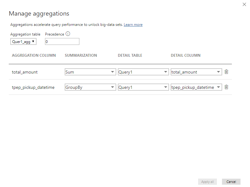
Use Case #4 – Aggregated table in DirectQuery mode
The next test will show us what happens if we create an aggregated table and store it in DirectQuery mode within the Power BI. It’s quite a simple aggregated table, consisting of total amount and pickup time columns.
My query hit the aggregated table, but it didn’t change anything in terms of the total query cost, as it was exactly the same like in the previous use case: ~0.02$!
Use Case #5 – Aggregated table in Import mode
After that, I want to check what happens if I import a previously aggregated table into Power BI. I believe that calculations will be faster, but let’s see how it will affect the query costs.
As expected, this was pretty quick, aggregated table was hit, so we are only paying the price of the data refresh, as in our Use Case #1: 0.018$!
Use Case #6 – Aggregated data in Serverless SQL pool
One last thing I want to check, is what happens if I know my analytic workloads, and can prepare some most frequent queries in advance, using Serverless SQL pool.
Therefore, I will create a view, that will aggregate the data like in the previous case within Power BI Desktop, but this time within the Serverless SQL pool:
DROP VIEW IF EXISTS taxi201901_02_agg;
GO

CREATE VIEW taxi201901_02_agg AS
  SELECT  CAST(C2 AS DATE) AS tpep_pickup_datetime,
        SUM(CAST(C17 AS DECIMAL(10,2))) AS total_amount
FROM
    OPENROWSET(
        BULK N'https://nikola.dfs.core.windows.net/nikola/Data/yellow_tripdata_2019-01.csv',
        FORMAT = 'CSV',
        PARSER_VERSION='2.0',
        HEADER_ROW = TRUE
    )
    AS [taxi201901_02_agg]
    GROUP BY CAST(C2 AS DATE)
Basically, we are aggregating data on the source side and that should obviously help. So, let’s check the outcome:

It returned requested figures faster, but the amount of the processed data was again the same! This query again costs me ~0.02$!
This brings me to a conclusion: no matter what you perform within the Serverless SQL pool on top of the CSV files, they will be fully scanned at the lowest level of the data preparation process!
However, and that’s important, it’s not just the scanned data amount that makes the total of the processed data, but also the amount of streamed data to a client: in my example, the difference between streamed data is not so big (275 MB when I’ve included all columns vs 1 MB when targeting aggregated data), and that’s why the final price wasn’t noticeably different. I assume that when you’re working with larger data sets (few TBs), the cost difference would be far more obvious. So, keep in mind that pre-aggregating data within a Serverless SQL pool can save you the amount of streamed data, which also means that your overall costs will be reduced! You can find all the details here.
Use Case #7 – Import Parquet files
Let’s now evaluate if something changes if we use data from Parquet files, instead of CSV.
The first use case is importing Parquet files. As expected, as they are better compressed than CSV files, costs decreased, almost by double: ~0.01$!
Use Case #8 – DirectQuery over Parquet files
And finally, let’s examine the figures if we use DirectQuery mode in Power BI to query the data directly from the Parquet files within the Serverless SQL pool in Synapse.
To my negative surprise, this query processed ~26 GB of data, which translates to ~0.13$!
As that looked completely strange, I started to investigate and found out that the main culprit for the high cost was the Date dimension created using M! While debugging the SQL query generated by Power BI and sent to SQL engine in the background, I’ve noticed that extremely complex query had been created, performing joins and UNION ALLs on every single value from the Date dimension:
SELECT
TOP (1000001) [semijoin1].[c1],SUM([a0])
 AS [a0]
FROM
(
(
SELECT [t1].[TpepPickupDatetime] AS [c13],[t1].[TotalAmount] AS [a0]
FROM
(
(SELECT *
FROM taxi201901parquet
UNION ALL
SELECT *
FROM taxi201902parquet)
)
 AS [t1]
)
 AS [basetable0]
 INNER JOIN
(
(SELECT 3 AS [c1],CAST( '20190101 00:00:00' AS datetime) AS [c13] )  UNION ALL
(SELECT 4 AS [c1],CAST( '20190102 00:00:00' AS datetime) AS [c13] )  UNION ALL
(SELECT 5 AS [c1],CAST( '20190103 00:00:00' AS datetime) AS [c13] )  UNION ALL
(SELECT 6 AS [c1],CAST( '20190104 00:00:00' AS datetime) AS [c13] )  UNION ALL
(SELECT 7 AS [c1],CAST( '20190105 00:00:00' AS datetime) AS [c13] )  UNION ALL
(SELECT 8 AS [c1],CAST( '20190106 00:00:00' AS datetime) AS [c13] )  UNION ALL
(SELECT 9 AS [c1],CAST( '20190107 00:00:00' AS datetime) AS [c13] )  UNION ALL
(SELECT 10 AS [c1],CAST( '20190108 00:00:00' AS datetime) AS [c13] )  UNION ALL
(SELECT 11 AS [c1],CAST( '20190109 00:00:00' AS datetime) AS [c13] )  UNION ALL
…..
This is just an excerpt from the generated query, I’ve removed rest of the code for the sake of readability.
Once I excluded my Date dimension from the calculations, costs expectedly decreased to under 400 MBs!!! So, instead of 26GB with the Date dimension, the processed data amount was now ~400MB!
To conclude, these scenarios using the Composite model need careful evaluation and testing.
Use Case #9 – Aggregated data in the Serverless SQL pool
That’s our tipping point! Here is where the magic happens! By being able to store columns physically separated, Parquet outperforms all previous use cases in this situation – and when I say this situation – I mean when you are able to reduce the number of necessary columns (include only those columns you need to query from the Power BI report).
Once I’ve created a view containing pre-aggregated data in the Serverless SQL pool, only 400 MB of data was processed! That’s an enormous difference comparing to all previous tests. Basically, that means that this query costs: 0.002$! For easier calculation – I can run it 500x to pay 1$!
Final Verdict
Here is the table with costs for every single use case I’ve examined:
| Use Case | Costs $ | Remark |
| Import CSV files in Power BI (2 visuals) | ~0.018 per refresh | Number of visuals and number of users don’t affect costs |
| DirectQuery over CSV files (2 visuals/1 user) | ~0.02 per 2 visuals/1 user | Number of visuals and number of users running report affect costs |
| Add Date slicer | ~0.02 | Same as previous |
| Aggregated table in DirectQuery mode (CSV) | ~0.02 per 2 visuals/1 user | Number of visuals and number of users running report affect costs |
| Aggregated table in Import mode (CSV) | ~0.018 per refresh | Number of visuals and number of users don’t affect costs |
| Aggregated data in Serverless SQL pool in Synapse (CSV) | ~0.02 per 2 visuals/1 user | Scans complete data from CSV files again. But, the streamed data amount is lower – makes the difference in larger datasets! |
| Import Parquet files in Power BI (2 visuals) | ~0.01 per refresh | Number of visuals and users don’t affect costs |
| DirectQuery over Parquet files | ~0.13 per 2 visuals/1 user with Date dim ** ~0.002 per 2 visuals/1 user without Date dim | Surprisingly high with Composite model (Date dim created using M and stored in Power BI)! Great results when Date dim was excluded |
| Aggregated data in Serverless SQL pool in Synapse (Parquet) | ~0.002 per 2 visuals/1 user | Magic! |
Looking at the table, and considering different use cases we’ve examined above, the following conclusions can be made:
- Whenever possible, use Parquet files instead of CSV
- Whenever possible, Import the data into Power BI – that means you will pay only when the data snapshot is being refreshed, not for every single query within the report
- If you are dealing with Parquet files, whenever possible, create pre-aggregated data (views) in the Serverless SQL pool in the Synapse
- Since Serverless SQL pool still doesn’t support ResultSet Cache (as far as I know, Microsoft’s team is working on it), keep in mind that each time you run the query (even if you’re returning the same result set), the query will be generated and you will need to pay for it!
- If your analytic workloads require a high number of queries over a large dataset (so large that Import mode is not an option), maybe you should consider storing data in the Dedicated SQL pool, as you will pay fixed storage costs then, instead of data processing costs each time you query the data. Here, in order to additionally benefit from using this scenario, you should materialize intermediate results using external tables, BEFORE importing them into a Dedicated SQL pool! That way, your queries will read already prepared data, instead of raw data
- Stick with the general best practices when using Serverless SQL pool within Synapse Analytics
Conclusion
In this article, we dived deep to test different scenarios and multiple use cases, when using Power BI in combination with the Serverless SQL pool in Synapse Analytics.
In my opinion, even though Synapse has a long way to go to fine-tune all the features and offerings within the Serverless SQL pool, there is no doubt that it is moving in the right direction. With constantly improving the product, and regularly adding cool new features, Synapse can really be a one-stop-shop for all your data workloads.
In the last part of this blog series, we will check how Power BI integrates with Azure’s NoSQL solution (Cosmos DB), and how the Serverless SQL pool can help to optimize analytic workloads with the assistance of Azure Synapse Link for Cosmos DB.
Thanks for reading!
Last Updated on November 20, 2020 by Nikola


Bob Dobalina
UNION ALL will return all records, UNION returns a unique set… think you might have the wrong way around