 Alberto Ferrari
UPDATE 2020-11-11: You can find more complete detailed and optimized examples for this calculation in the DAX Patterns: Transition matrix article+video on daxpatterns.com.
Ranking is an important part of any business. You might rank your customers, or products, or any business asset using some rule. In this example, we use a very simple ranking based on the amount sold on a yearly basis. To perform this action, we use this table:
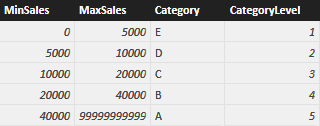
Category E is the worst, and customers in category are rated 1 (lowest value), whereas customers in category A are the best and are valued 5. You typically store such a table in SQL but, because the article is about calculated tables, I prefer to create it using the following DAX code:
SaleCategory =
UNION (
    ROW ( "MinSales",     0, "MaxSales",        5000, "Category", "E", "CategoryLevel", 1 ),
    ROW ( "MinSales",  5000, "MaxSales",       10000, "Category", "D", "CategoryLevel", 2 ),
    ROW ( "MinSales", 10000, "MaxSales",       20000, "Category", "C", "CategoryLevel", 3 ),
    ROW ( "MinSales", 20000, "MaxSales",       40000, "Category", "B", "CategoryLevel", 4 ),
    ROW ( "MinSales", 40000, "MaxSales", 99999999999, "Category", "A", "CategoryLevel", 5 )
)
Once the table is in the model, you cannot create a relationship between it and the customers, because the category of the customer changes every year. This looks the perfect scenario for dynamic segmentation and in fact, if you are only interested in a purely dynamic segmentation, you can follow that well-known pattern.
Instead, you are interested in verifying how the category of customers evolves over time, using a transition matrix for such attribute. If, for example, a customer had an A in 2008 and a D in 2009, then it became a worse buyer, and you want to understand how many of your customers are moving from one category to another or, given a group of customers, whether their ranking is increasing or decreasing, on average.
You can solve the scenario with pure DAX code, by authoring some rather complex measures. For example, you can compute the category level of a customer in the current and in the previous year using these two measures:
Customer[CatLevel] :=
VAR
    SalesCurrentYear = [Sales Amount]
RETURN
    CALCULATE (
        VALUES ( SaleCategory[CategoryLevel] ),
        SaleCategory[MinSales] < SalesCurrentYear,
        SaleCategory[MaxSales] >= SalesCurrentYear
    )
Customer[CatLevelLastYear] :=
VAR SalesLastYear =
    CALCULATE (
        [Sales Amount],
        SAMEPERIODLASTYEAR ( 'Date'[Date] ),
        ALL ( 'Date' )
    )
RETURN
    CALCULATE (
        VALUES ( SaleCategory[CategoryLevel] ),
        SaleCategory[MinSales] < SalesLastYear,
        SaleCategory[MaxSales] >= SalesLastYear
    )
Once the two measures are in place, you can simply compute an AVERAGEX on Customer of the difference between the two, in order to compute the average variation in category:
AvgVariation := AVERAGEX ( Customer, [CatLevel] – [CatLevelLastYear] )
Obviously, you would need to add some conditional logic in the special case where the customer did not exist in the previous year because, in such a case, you would compute a wrong variation. These measures are neither utterly complicated nor slow but, for large datasets, they use a lot of CPU because they need to compute the same value again and again. Moreover, this only solves the problem of computing the average variation but, if you are interested in counting the number of customers who moved from one category to another one, then you need to roll up your sleeves and:
- Create two dummy dimensions: one for the category the customer had the year before and one for the category the customer had this year
- Use a variation of the dynamic segmentation pattern to compute the number of customers in each segment, using the previous or current category chosen from one of the previous technical dimensions
It is pointless to provide the full solution in this article, our interest on this is only to say that the solution, although existing, is a complex one and the speed of these calculations is not top-notch.
A much better approach is that of creating a table containing all the needed information in a single place, namely:
- Customer Name
- Calendar Year
- Category and level in the given year
- Category and level in the previous year
Such a table has many advantages:
- It is much smaller than the fact table, its size will be Customers x Years
- It already contains, although denormalized, the current and previous category, making the two dummy dimensions useless
- It makes the calculation of the average variation a simple AVERAGE, making also it possible to compute the average over multiple years
- Because it contains the customer key, it relies on physical relationships to perform slicing by customer attributes, resulting in pure storage engine queries
This is a perfect example where a DAX calculated table fits just fine. You can write a query that computes such a table using the following code:
CustomerCategoryByTear =
ADDCOLUMNS (
    GENERATE (
        GENERATE (
            ADDCOLUMNS (
                SUMMARIZE (
                    Sales,
                    Customer[CustomerKey],
                    'Date'[Calendar Year]
                ),
                "SalesInYear", [Sales Amount],
                "SalesInPreviousYear", CALCULATE (
                    [Sales Amount],
                    SAMEPERIODLASTYEAR ( 'Date'[Date] ),
                    ALL ( 'Date' )
                )
            ),
            CALCULATETABLE (
                SELECTCOLUMNS (
                    SaleCategory,
                    "CategoryLevel", SaleCategory[CategoryLevel],
                    "Category", SaleCategory[Category]
                ),
                FILTER (
                    SaleCategory,
                    AND (
                        SaleCategory[MinSales] < [SalesInYear],
                        SaleCategory[MaxSales] >= [SalesInYear]
                    )
                )
            )
        ),
        CALCULATETABLE (
            SELECTCOLUMNS (
                SaleCategory,
                "CategoryLevelPreviousYear", SaleCategory[CategoryLevel],
                "CategoryPreviousYear", SaleCategory[Category]
            ),
            FILTER (
                SaleCategory,
                AND (
                    SaleCategory[MinSales] < [SalesInPreviousYear],
                    SaleCategory[MaxSales] >= [SalesInPreviousYear]
                )
            )
        )
    ),
    "Delta", ( [CategoryLevel] - [CategoryLevelPreviousYear] )
)
There are a few interesting points in this query:
- By using GENERATE instead of GENERATEALL, we are implicitly removing all rows where the customer is not categorized in both years. The query only computes effective variations in ranking, avoiding the special cases where a customer completely stops buying (it does not have a category in the current year) or he is a new customer (it does not have a category in the previous year)
- Using GENERATE and SELECTCOLUMNS, you can compute the category and its level with a single lookup
- Please note that we avoided (it is a best practice) to use SUMMARIZE to compute Sales and SalesLastYear. Instead, we used the pair of ADDCOLUMNS and SUMMARIZE to obtain better speed and safe results
We used the Contoso database to test the measure. The fact table contains 12M rows whereas the table resulting from this query only contains 35K rows. As a natural consequence, querying this table results in great performance and you can easily build a matrix like the following one, that shows how many customers belong to each category and year and from which category they come:
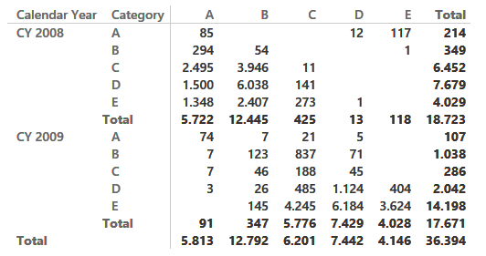
Because the matrix shows only variations, numbers might look wrong at first sight. For instance, there are 4,029 customers in class E in 2008 but only 4,028 moved to a different category in 2009, one is a completely lost customer and does not appear in this report).
If you are interested in the average variation of customers, you can easily build the AVERAGE of Delta and show it on a matrix like the following one ( showing the average variation per country and year) with a nice average variation over all the years shown in the Total column:
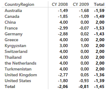
The model might well be improved by assigning a negative impact on lost customers and a positive one to new customers, so to show a better representation of the business, but this requires a better definition of the metrics, and is out of scope for a purely technical article.
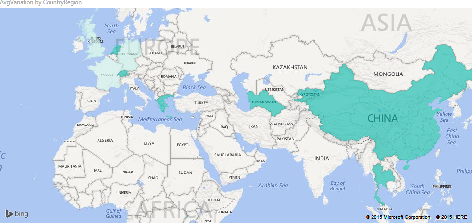
Needless to say, with Power BI you can project the same information on a map, providing a better impact to your presentations:
There are many more scenarios where calculated tables shine, the limit is only your imagination. Calculated columns are useful to persist single numbers, whereas the power of calculated tables is that they can persist entire tables at different granularities, highly reducing the need to write ETL code in your solutions.
Unfortunately, calculated tables are not available in Excel 2016. If you need a similar solution with Excel 2016, you can rely on linked back tables (i.e. queries over the data model materialized in Excel tables and then loaded back in the model). The only limitation is that the size of linked back tables cannot exceed the physical limit of 1M rows of Excel, whereas DAX calculated tables have no limit in size and can work in many more scenarios, resulting in a very elegant and neat model.
Calculates the average (arithmetic mean) of a set of expressions evaluated over a table.
AVERAGEX ( <Table>, <Expression> )
Returns the average (arithmetic mean) of all the numbers in a column.
AVERAGE ( <ColumnName> )
The second table expression will be evaluated for each row in the first table. Returns the crossjoin of the first table with these results.
GENERATE ( <Table1>, <Table2> )
The second table expression will be evaluated for each row in the first table. Returns the crossjoin of the first table with these results, including rows for which the second table expression is empty.
GENERATEALL ( <Table1>, <Table2> )
Returns a table with selected columns from the table and new columns specified by the DAX expressions.
SELECTCOLUMNS ( <Table> [[, <Name>], <Expression> [[, <Name>], <Expression> [, … ] ] ] )
Creates a summary of the input table grouped by the specified columns.
SUMMARIZE ( <Table> [, <GroupBy_ColumnName> [, [<Name>] [, [<Expression>] [, <GroupBy_ColumnName> [, [<Name>] [, [<Expression>] [, … ] ] ] ] ] ] ] )
Returns a table with new columns specified by the DAX expressions.
ADDCOLUMNS ( <Table>, <Name>, <Expression> [, <Name>, <Expression> [, … ] ] )