 Alberto Ferrari
UPDATE 2021-11-07: The terms “strong” and “weak” relationships used in a previous version of this article have been replaced by “regular” and “limited” relationship, respectively. These are the names used in the Microsoft documentation after the original article was published, we now aligned this article to the existing Microsoft terminology. You can find other content using the terms “strong” and “weak” relationships. That content is still valid, just consider that a “strong” relationship is now a regular relationship and a “weak” relationship is now a limited relationship. Specifically, in this article we kept the name of tables and measures in the sample files and using the “strong” and “weak” terms, but they correspond to “regular” and “limited” concepts explained in the article.
Limited relationships were introduced in Power BI with composite models in 2018. Even though they look like regular relationships, they hide some complexities. These relationships are part of the Tabular model, though as of September 2019 it is not possible to use composite models in Analysis Services. Nevertheless, Analysis Services 2019 makes it possible to use limited relationships without using composite models, so this article is relevant to any future Tabular model that could use limited relationships. For this reason, when the article references the “Tabular model” the concepts can be applied to both Power BI and Analysis Services.
A relationship in a Tabular model can either be regular or limited. In a regular relationship the engine knows that the one-side of the relationship contains unique values. If the engine cannot ensure that the one-side of the relationship contains unique values for the key, then the relationship is limited. A relationship can be limited either because the engine cannot ensure the uniqueness of the constraint – due to technical reasons we shall outline later – or because the developer defined it as such. A limited relationship is not used as part of table expansion. Let us elaborate on this.
Power BI can create composite models. A composite model can contain tables both in Import mode (a copy of the data from the data source is preloaded and cached in memory using VertiPaq) and in DirectQuery mode (the data source is accessed only at query time). From hereinafter we use VertiPaq as an alias for Import mode and DirectQuery as short for DirectQuery mode.
A single data model can have tables stored in VertiPaq and others stored in DirectQuery. Moreover, tables in DirectQuery can originate from different data sources, generating several DirectQuery data islands.
In order to differentiate between data in VertiPaq and data in DirectQuery, we talk about data in the continent (VertiPaq) or in the islands (DirectQuery data sources).
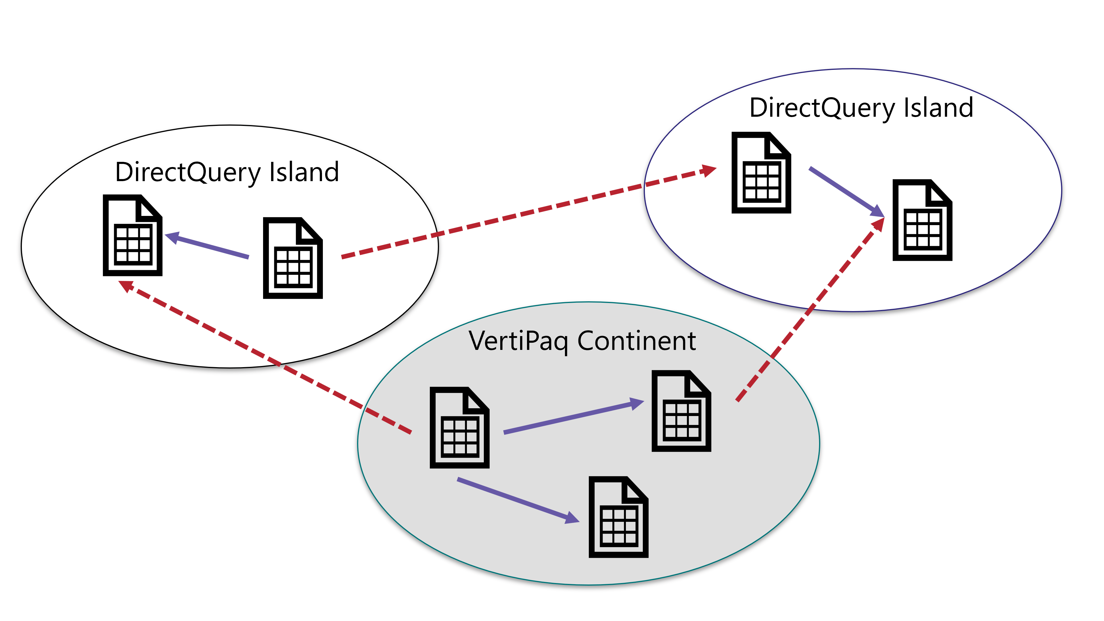
The VertiPaq store is nothing but another data island. We call it the continent only because it is the most frequently used data island. A relationship links two tables, and these two tables can belong to any island. If both tables belong to the same island, then the relationship is an intra-island relationship. If the two tables belong to different islands, then it is a cross-island relationship.
When a table is stored in the continent, the engine has full access to its content. Therefore, all the intra-island relationships in the continent are materialized at data refresh time. Indeed, a relationship is one of several internal structures created by the VertiPaq engine as part of the processing. A relationship is a data structure optimized to join two tables at query time in the most efficient way.
When a table is in DirectQuery mode, the engine does not have access to the table data itself. At query time, it will execute a query on the database hosting the table to gather the required information. Nevertheless, the DAX engine does not read the content of the table at data refresh time. Moreover, even though the DAX engine reads the data in the table, the data could change at any time. In other words, the engine cannot make any assumption about the table content. Therefore, the DAX engine cannot ensure unique values in the primary key of the table that is the target of a relationship.
An intra-island relationship on a data island other than the continent can be solved by the data source provider of the island itself, by sending appropriate JOIN and WHERE clauses to the data island engine. In a query, tables linked through an intra-island relationship will be joined together by the storage engine of the island itself. Therefore, the DAX formula engine does not need to perform the join, as it trusts the storage engine to execute it. VertiPaq intra-island relationships are usually regular relationships, enforced and handled by the VertiPaq storage engine; explicit limited relationships in VertiPaq are the exception described later.
The most complex scenario happens with cross-island relationships. A cross-island relationship links two tables that are stored in different data sources. As such, the relationship needs to be resolved by the DAX formula engine, which will read the relevant information from the two data sources and then join the tables. A cross-island relationship is the first kind of limited relationship.
A similar scenario happens when you create a relationship between two tables and the column used to build the relationship is not unique in both tables. In that case, the relationship has a many-to-many cardinality and, even though it is a relationship within the continent, it is always a limited relationship.
Therefore, a relationship is limited if it has a many-to-many cardinality or if it is a cross-island relationship.
We are not going to discuss why one would choose one type of relationship over another. The choice between different types of relationships and filter propagation is in the hands of the data modeler; their decision flows from a deep reasoning on the semantics of the model itself. From a DAX point of view, limited and regular relationships behave differently, and it is important to understand the differences among the relationships and the impact they have on the DAX code.
When two tables are linked through a regular relationship, the table on the one-side might contain the additional blank row in case the relationship is invalid. Thus, if the many-side of a regular relationship contains values that are not present in the table on the one-side, then a blank row is appended to the one-side table. The additional blank row is not added to the target of a limited relationship.
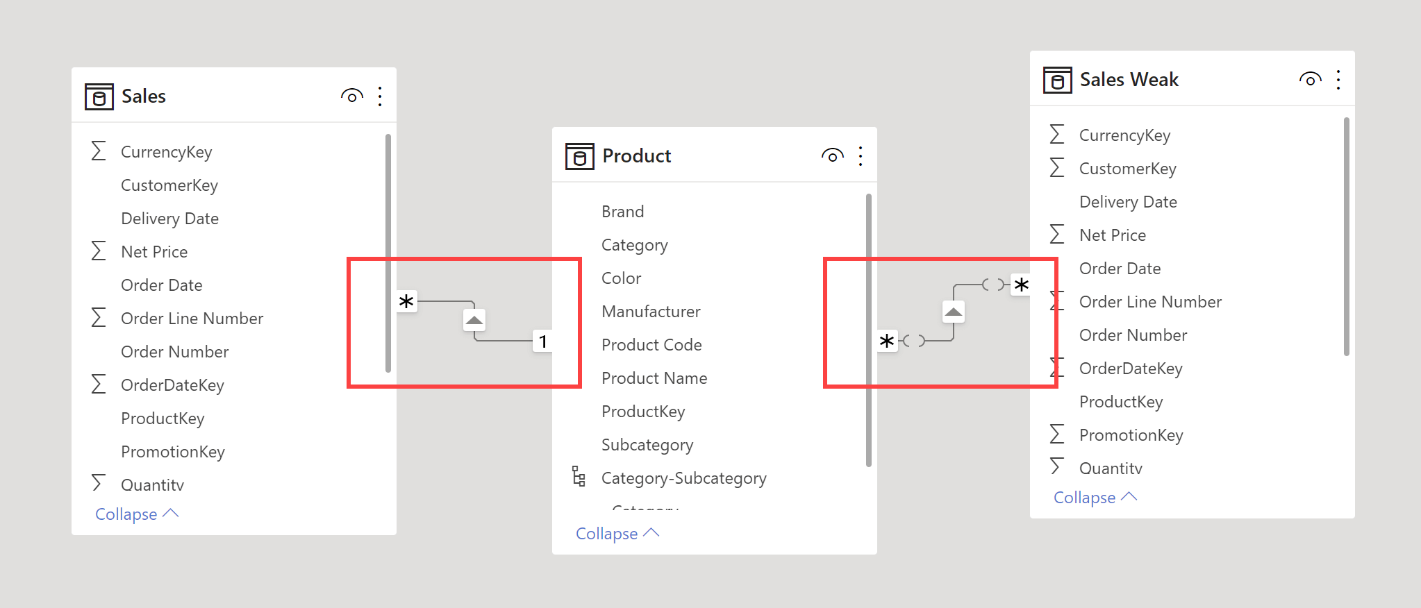
This can be the source of rather surprising behavior. As an example, look at the following model: there are two identical copies of the Sales table, but the relationship between Product and Sales is regular, whereas the relationship between Product and Sales Weak is defined with a many-to-many cardinality, therefore it is a limited relationship. Beware: there is no reason to define the relationship as such. It is a regular one-to-many relationship, we just used the many-to-many cross-filter to force the relationship to be limited in the continent.
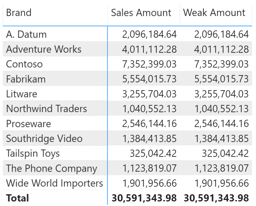
If we slice Sales and Sales Weak by Product[Brand], the numbers are – as expected – identical.
Right now, there is no blank row in the Product table. In order to force the creation of the blank row, we deleted from the Product table all the products of the Wide World Importers brand. The result is surprising.
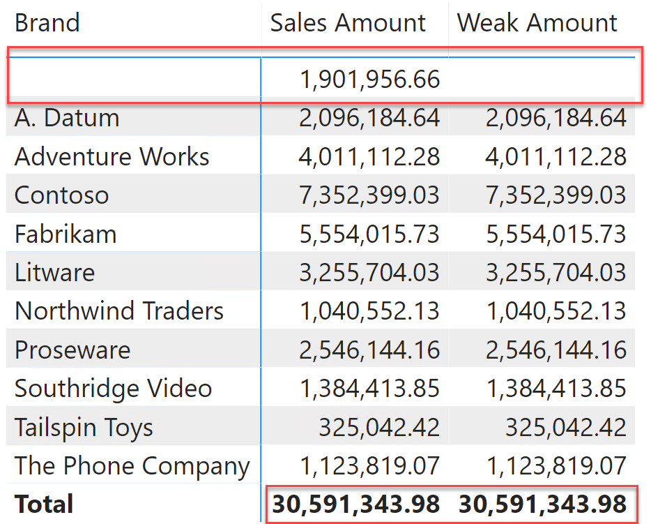
You should note two things in the previous figure. The Product table now contains the blank row, which accounts for the missing brand. Nevertheless, no revenues in the Weak Amount measure are related to the blank row, because blank row links are not enforced through limited relationships. All the values being identical, you can easily check that the total shown for Weak Amount is different than the sum of individual brands.
As we anticipated, in the example we have artificially marked the relationship with the Weak Sales table as limited. Nevertheless, this is the expected behavior for any limited relationship, mostly important when the relationship is limited despite being a regular intra-island one-to-many relationship.
Another important difference is that table expansion does not work through limited relationships. This is not a big issue, unless you are a DAX guru. Indeed, there are few scenarios where table expansion is used in DAX: If you are using table expansion in any of your DAX formulas, you are expected to already know quite well how relationships affect table expansion. If not, then be careful because you are playing with fire!
Finally, another important difference between regular and limited relationships is in performance. Regular relationships are materialized during data refresh by building optimized data structures that reduce the cost of joining tables at query time. These data structures are not created for limited relationships.
To demonstrate this, we executed two similar queries – first querying the Sales table and then querying the Weak Sales table:
EVALUATE
VAR OneCategory =
    TREATAS ( { "Audio" }, 'Product'[Category] )
RETURN
    SUMMARIZECOLUMNS (
        'Product'[Category],
        OneCategory,
        "Test", [Sales Amount]
    )
When executed using Sales as the target, the relationship is regular. Therefore, the engine can rely on its internal structures and the query plan generates a very simple VertiPaq query:
WITH $Expr0 :=
    ( PFCAST ( 'Sales'[Quantity] AS  INT ) * PFCAST ( 'Sales'[Net Price] AS  INT )  )
SELECT
    SUM ( @$Expr0 ) FROM 'Sales'
LEFT OUTER JOIN 'Product'
    ON 'Sales'[ProductKey]='Product'[ProductKey]
    WHERE 'Product'[Category] = 'Audio'
As you can see, the join between the two tables is handled inside the VertiPaq engine.
When we replace the Sales Amount measure reference with Weak Amount, the query is similar but the query plan is more complex:
EVALUATE
VAR OneCategory =
    TREATAS ( { "Audio" }, 'Product'[Category] )
RETURN
    SUMMARIZECOLUMNS (
        'Product'[Category],
        OneCategory,
        "Test", [Weak Amount]
    )
This time the query plan executes three different VertiPaq queries. First, it gathers the values of ProductKey corresponding to the Audio category:
DEFINE TABLE '$TTable3' :=
SELECT
    'Product'[ProductKey], 'Product'[Category]
FROM
    'Product'
WHERE
    'Product'[Category] = 'Audio'
Then, there is a request to build a bitmap of ProductKey values that are present in the Sales Weak table:
DEFINE TABLE '$TTable4' :=
SELECT
    RJOIN ( '$TTable3'[Product$ProductKey] )
FROM '$TTable3'
    REVERSE BITMAP JOIN 'Sales Weak'
    ON '$TTable3'[Product$ProductKey]='Sales Weak'[ProductKey];
Finally, the query plan gathers Sales by ProductKey, and it uses $TTable3 to map ProductKey to Category:
DEFINE TABLE '$TTable1' :=
SELECT
    '$TTable3'[Product$Category],
    SUM ( '$TTable2'[$Measure0] )
FROM '$TTable2'
    INNER JOIN '$TTable3' ON '$TTable2'[Sales Weak$ProductKey]='$TTable3'[Product$ProductKey]

REDUCED BY
    '$TTable2' := WITH
        $Expr0 := ( PFCAST ( 'Sales Weak'[Quantity] AS  INT ) * PFCAST ( 'Sales Weak'[Net Price] AS  INT )  )

    SELECT
        'Sales Weak'[ProductKey], SUM ( @$Expr0 )
    FROM 'Sales Weak'
    WHERE
        'Sales Weak'[ProductKey] ININDEX '$TTable4'[$SemijoinProjection];
This query approach – the slowest of them all – is still extremely fast on the sample model related to this article that you can download. Nevertheless, this approach requires multiple scans of the fact table – one to perform the RJOIN and one to gather the actual value for sales amount – and its complexity depends on the size of the product table. The larger the number of products, the slower the query. This is the reason why you can safely rely on limited relationships if the cardinality of the column used to join the two tables is pretty small (up to 100/200 unique values). Larger cardinality columns tend to be slow and should be treated with much care.
Power BI has different visual representations for regular and limited relationships. While the regular relationship between Product and Sales has a regular line connecting the two tables, the limited relationship between Product and Sales Weak has separations in the line, close to each table. Those “disconnected” graphical elements represent the limited relationship role.
Regular and limited relationships provide more flexibility in designing Tabular models, even though you should be aware of the different behavior in case of missing keys on the one-side of a relationship. As usual, DAX is simple, but it is not easy.