Relationships in Power BI and Tabular models

UPDATE 2021-11-04: The terms “strong” and “weak” relationships used in a previous version of this article have been replaced by “regular” and “limited” relationship, respectively. These are the names used in the Microsoft documentation after the original article was published, we now aligned this article to the existing Microsoft terminology. You can find other content using the terms “strong” and “weak” relationships. That content is still valid, just consider that a “strong” relationship is now a regular relationship and a “weak” relationship is now a limited relationship.

Power BI and Analysis Services rely on a semantic model based on the Tabular Object Model (TOM). Even though there are different tools to manipulate these models – we suggest using Tabular Editor – the underlying concepts are identical because the engine and the data model is the same: we call it the Tabular model. This article is based on a section of The Definitive Guide to DAX (second edition) and on the Different types of many-to-many relationships in Power BI video.

In a Tabular model, a physical relationship connects two tables through an equivalence over a single column. Under certain conditions that we will be describing later, a relationship can define a constraint on the content of a table, even though such constraint is different from the “foreign key constraint” many SQL developers are used to. However, the purpose of a relationship in a Tabular model is to transfer a filter while querying the model. Because transferring a filter is also possible by writing DAX code, we define two categories of relationships:

Virtual relationships: these are relationships that are not defined in the data model but can be described in the logical model. Virtual relationships are implemented through DAX expressions that transfer the filter context from one table to another. A virtual relationship can rely on more than one column and can be related to a logical expression that is not just a column identity. Virtual relationships can be used to define multi-column relationships and relationships based on a range.
Physical relationships: these are the relationships defined in a Tabular model. The engine automatically propagates the filter context in a query according to the filter direction of the active relationship. Inactive relationships are ignored, but there are DAX functions that can manipulate the state and the filter direction of physical relationships: USERELATIONSHIP and CROSSFILTER.

In this article we first show virtual relationships. We then discuss in detail the different types of physical relationships, also introducing the concept of limited relationships. Finally, we introduce many-to-many relationships, describing the different kinds of many-to-many relationships available in a model and in Power BI, thus clarifying the differences between the available options and briefly discussing performance implications.

Virtual relationships

A virtual relationship is a filter applied to the filter context in a CALCULATE or CALCULATETABLE function. In order to propagate a filter from A to B, you have to read the values active in the filter context on A and apply a corresponding filter to B.

For example, imagine having to transfer the filter from Customer to Sales. The optimal way to do this is by using TREATAS:

CALCULATE (
    [measure],
    TREATAS ( 
        VALUES ( Customer[CustomerKey] ), -- Read filter from Customer
        Sales[CustomerKey]                -- Apply filter to Sales
    )
)

The TREATAS function can also implement a logical relationship based on multiple columns. For example, the following code transfers the filter from a Sales table over to a Delivery table using Order Number and Order Line Number:

CALCULATE (
    [measure],
    TREATAS ( 
        SUMMARIZE ( 
            Sales,
            Sales[Order Number],      -- Read filter from Sales
            Sales[Order Line Number]  -- based on multiple columns
        ),
        Delivery[Order Number],       -- Apply filter to Delivery 
        Delivery[Order Line Number]   -- specifying corresponding columns
    )
)

NOTE: creating a virtual relationship based on multiple columns is not optimal from a performance standpoint. A physical, single-column relationship is orders of magnitude faster than a virtual relationship.

Because TREATAS is a relatively new function, there are other common techniques used in order to implement virtual relationships. We include these alternatives as a reference; Remember that TREATAS is the preferred way to create a virtual relationship based on column equivalency.

The first alternative technique is using INTERSECT:

CALCULATE (
    [measure],
    INTERSECT ( 
        ALL ( Sales[CustomerKey] ),       -- Apply filter to Sales
        VALUES ( Customer[CustomerKey] ), -- Read filter from Customer
    )
)

The second alternative technique is using IN:

CALCULATE (
    [measure],
    Sales[CustomerKey] IN VALUES ( Customer[CustomerKey] )
)

Another alternative technique is using FILTER and CONTAINS, which is older and slower than INTERSECT:

CALCULATE (
    [measure],
    FILTER ( 
        ALL ( Sales[CustomerKey] ),           -- Apply filter to Sales
        CONTAINS (
            VALUES ( Customer[CustomerKey] ), -- Read filter from Customer
            Customer[CustomerKey], 
            Sales[CustomerKey] 
        )
    )
)

A virtual relationship can be based on a range, like the technique used to implement a dynamic segmentation:

CALCULATE (
    [measure],
    FILTER ( 
        ALL ( Sales[Net Price] ),  -- Apply filter to Sales
        NOT ISEMPTY (              -- filtering prices
            FILTER (               -- within the active ranges
                PriceRange,
                PriceRange[Min Price] <= Sales[Net Price]
                    && Sales[Net Price] < PriceRange[Max Price]
            )
        )
    )
)

Physical relationships

A relationship can be regular or limited. In a regular relationship the engine knows that the one-side of the relationship contains unique values. If the engine cannot check that the one-side of the relationship contains unique values for the key, then the relationship is limited. A relationship can be limited either because the engine cannot ensure the uniqueness of the constraint, due to technical reasons we outline later, or because the developer defined it as such.

A limited relationship is not used as part of table expansion. Power BI has been allowing composite models since 2018; In a composite model, it is possible to create tables in a model containing data in both Import mode (a copy of data from the data source is preloaded and cached in memory using the VertiPaq engine) and in DirectQuery mode (the data source is only accessed at query time).

A single data model can contain tables stored in VertiPaq and tables stored in DirectQuery. Moreover, tables in DirectQuery can originate from different data sources, generating several DirectQuery data islands.

In order to differentiate between data in VertiPaq and data in DirectQuery, we say that data is either in the continent (VertiPaq) or in the islands (DirectQuery data sources).

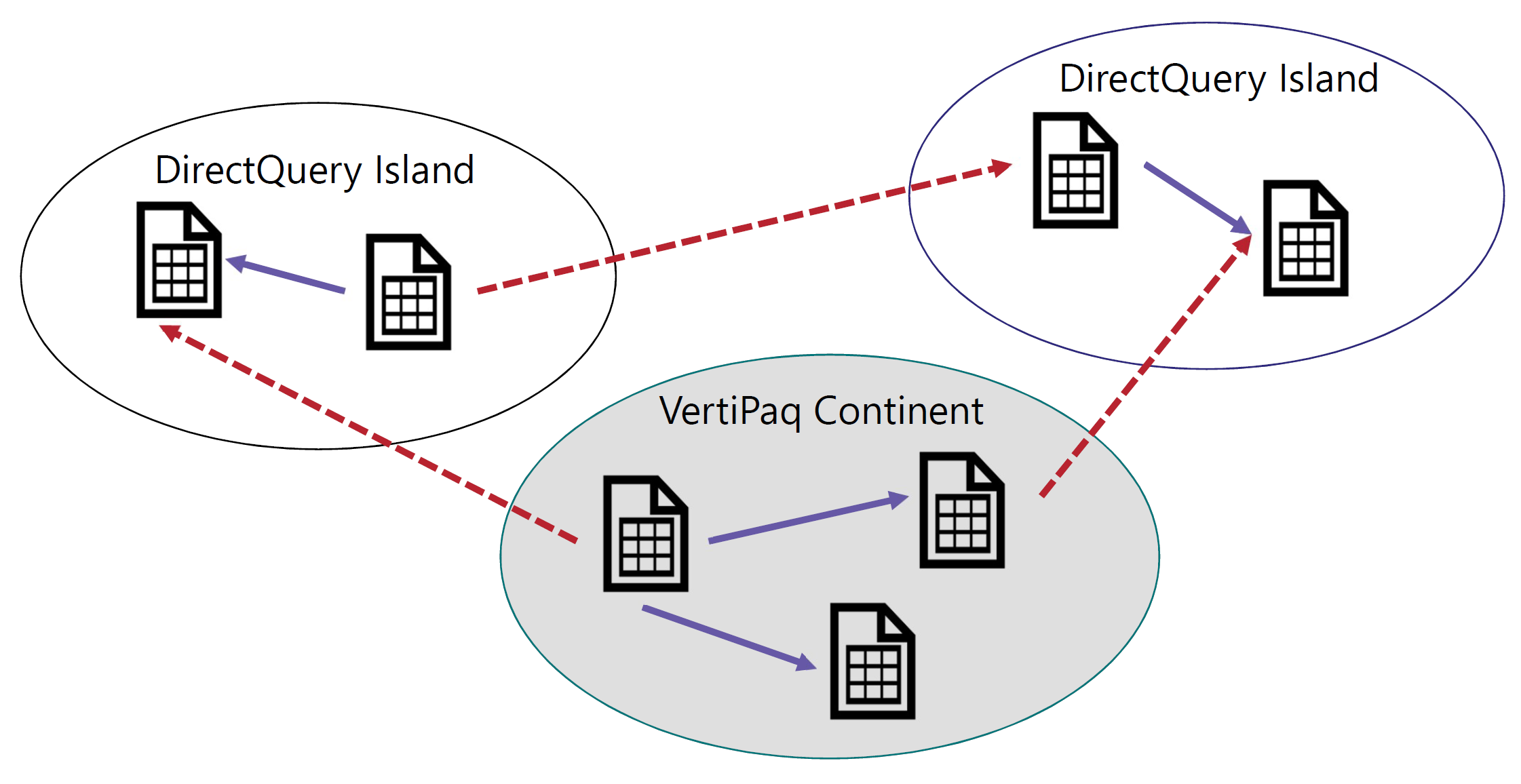
The VertiPaq store is nothing but another data island. We call it the continent only because it is the most frequently used data island.

A relationship links two tables. If both tables belong to the same island, then the relationship is an intra-island relationship. If the two tables belong to different islands, then it is a cross-island relationship. Cross-island relationships are always limited relationships. Therefore, table expansion never crosses islands.

Relationships have a cardinality, of which there are three types. The difference between them is both technical and semantical. Here we do not cover the reasoning behind those relationships because it would involve many data modeling digressions that are outside of the scope of this article. Instead, we need to cover the technical details of physical relationships and the impact they have on the DAX code.

These are the three types of relationship cardinality available:

One-to-many relationships: This is the most common type of relationship cardinality. On the one-side of the relationship the column must have unique values; on the many-side the value can (and usually does) contain duplicates. Some client tools differentiate between one-to-many relationships and many-to-one relationships. Still, they are the same type of relationship. It all depends on the order of the tables: a one-to-many relationship between Product and Sales is the same as a many-to-one relationship between Sales and Product.
One-to-one relationships: This is a rather uncommon type of relationship cardinality. On both sides of the relationship the columns need to have unique values. A more accurate name would be “zero-or-one”-to-“zero-or-one” relationship because the presence of a row in one table does not imply the presence of a corresponding row in the other table.
Many-to-many relationships: On both sides of the relationship the columns can have duplicates. This feature was introduced in 2018, and unfortunately its name is somewhat confusing. Indeed, in common data modeling language “many-to-many” refers to a different kind of implementation, created by using pairs of one-to-many and many-to-one relationships. It is important to understand that in this scenario many-to-many does not refer to the many-to- many relationship, but instead to the many-to-many cardinality of the relationship.

In order to avoid ambiguity with the canonical terminology which uses many-to-many for a different kind of implementation, we use acronyms to describe the cardinality of a relationship:

One-to-many relationships: We call them SMR, which stands for Single-Many-Relationship.
One-to-one relationships: We use the acronym SSR, which stands for Single-Single-Relationship.
Many-to-many relationships: We call them MMR, which stands for Many-Many-Relationship.

Another important detail is that an MMR relationship is always limited, regardless of whether the two tables belong to the same island or not. If the developer defines both sides of the relationship as the many-side, then the relationship is automatically treated as a limited relationship with no table expansion taking place.

In addition, each relationship has a cross-filter direction. The cross-filter direction is the direction used by the filter context to propagate its effect. The cross-filter can be set to one of two values:

Single: The filter context is always propagated in one direction of the relationship and not the other way around. In a one-to-many relationship, the direction is always from the one-side of the relationship to the many-side. This is the standard and most desirable behavior.
Both: The filter context is propagated in both directions of the relationship. This is also called a bidirectional cross-filter and sometimes just a bidirectional relationship. In a one-to-many relationship, the filter context still retains its feature of propagating from the one-side to the many-side, but it also propagates from the many-side to the one-side.

The cross-filter directions available depend on the type of relationship.

In an SMR relationship one can always choose single or bidirectional.
An SSR relationship always uses bidirectional filtering. Because both sides of the relationship are the one-side and there is no many-side, bidirectional filtering is the only option available.
In an MMR relationship both sides are the many-side. This scenario is the opposite of the SSR relationship: Both sides can be the source and the target of a filter context propagation. Thus, one can choose the cross-filter direction to be bidirectional, in which case the propagation always goes both ways. Or if the developer chooses single propagation, they also must choose which table to start the filter propagation from. As with all other relationships, single propagation is the best practice.

The following table summarizes the different types of relationships with the available cross-filter directions, their effect on filter context propagation, and the options for limited/regular relationship.

Type of Relationship	Cross-filter Direction	Filter Context Propagation	Limited & Regular Type
SMR	Single	From one-side to many-side	Limited if cross-island, regular otherwise
SMR	Both	Bidirectional	Limited if cross-island, regular otherwise
SSR	Both	Bidirectional	Limited if cross-island, regular otherwise
MMR	Single	Must choose the source table	Always limited
MMR	Both	Bidirectional	Always limited

When two tables are linked through a regular relationship, the table on the one-side might contain the additional blank row in case the relationship is invalid –VertiPaq Analyzer reports a Referential Integrity violation when this happens. Thus, if the many-side of a regular relationship contains values not present in the table on the one-side, then a blank row is appended to the table on the one-side. The additional blank row is never added to tables involved in a limited relationship.

A physical relationship can automatically propagate a filter in the filter context based on the filter propagation direction. Moreover, a relationship defines a unique constraint on columns that are on the one-side of a relationship.

Many-to-many relationships between business entities aka dimensions

A logical many-to-many relationship between two tables representing two different business entities –also known as dimension tables in dimensional modeling – cannot be implemented using a single physical relationship.

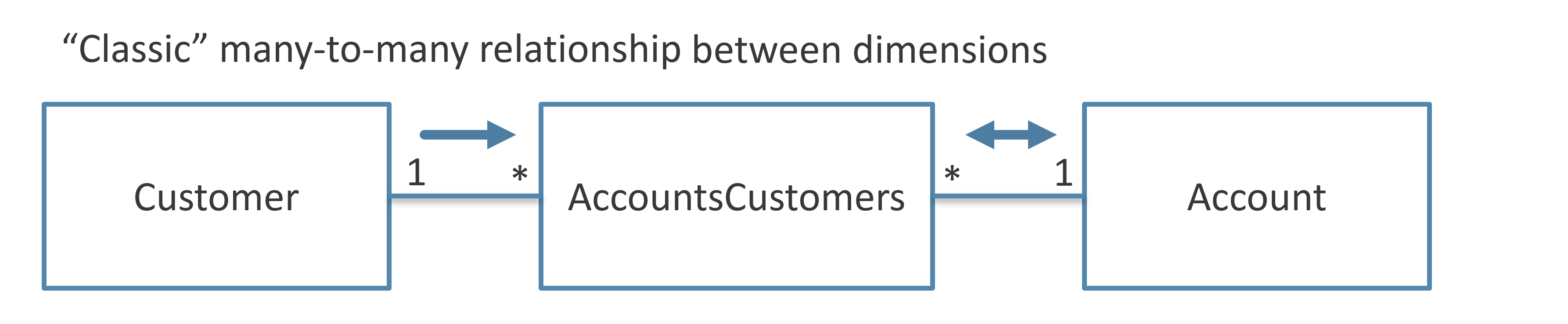
For example, consider the case of two tables, Customer and Account in a bank. Every customer can have multiple accounts, and every account can be owned by several customers. The relationship between the Customer and Account tables requires a third table, AccountsCustomers, which contains one row for each existing relationship between Account and Customer.

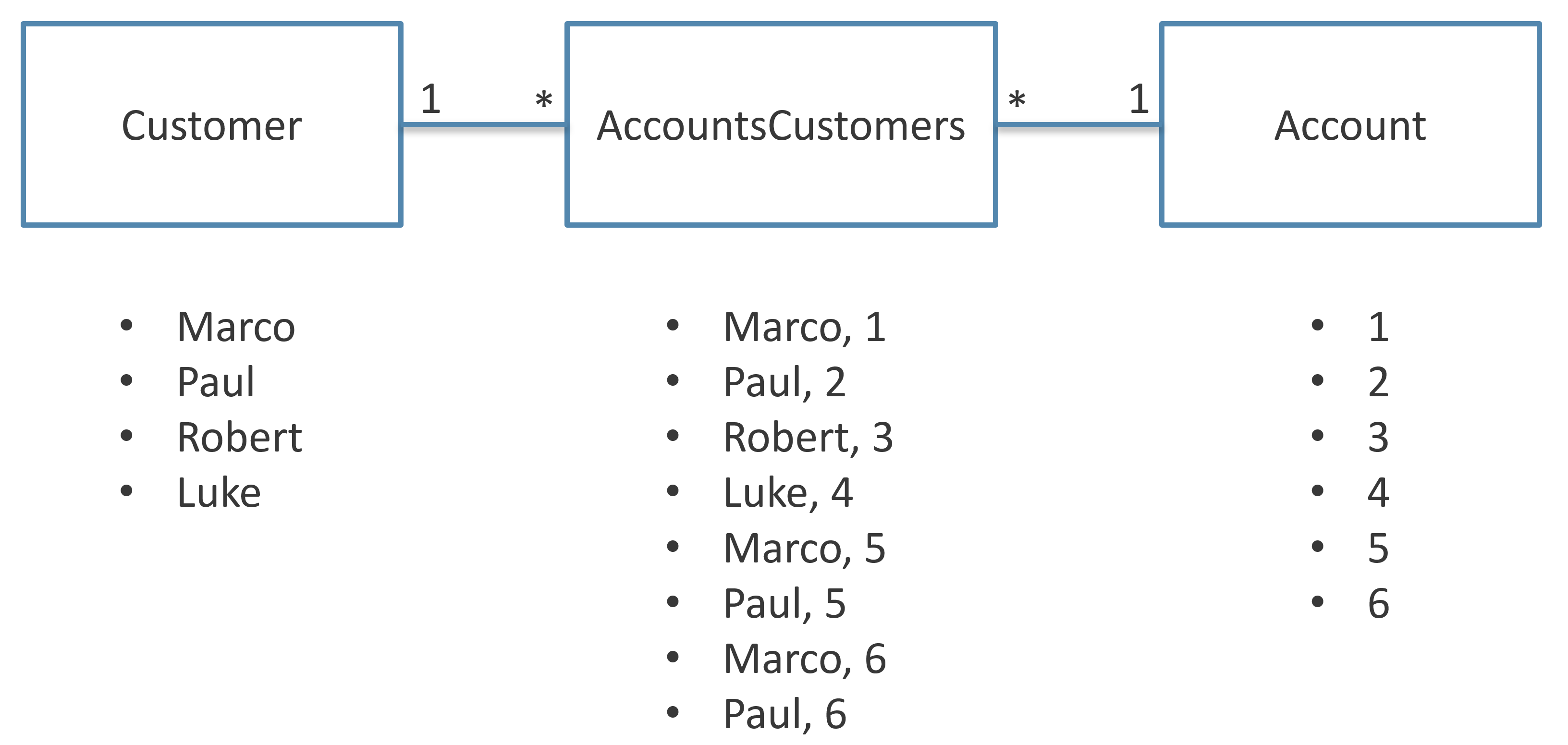
The logical many-to-many relationship between Customer and Account is implemented through two physical SMR relationships. In order to enable the propagation of the filter context from Customer to Account, a bidirectional filter must be activated in the data model on the relationship between Customer and AccountsCustomers.

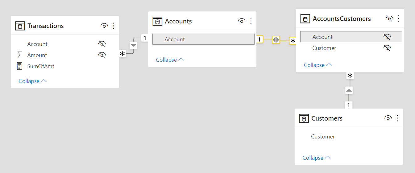
However, in order to avoid ambiguity caused by bidirectional filters in the data model, it is considered best practice to enable the bidirectional filter only in DAX measures that require that filter propagation. For example, if the relationship between Customer and AccountsCustomers is defined with a single direction filter, the bidirectional filter can be activated using CROSSFILTER as in the following measure:

SumOfAmt := 
CALCULATE ( 
    SUM ( Transactions[Amount] ), 
    CROSSFILTER ( 
        AccountsCustomers[AccountKey], 
        Accounts[AccountKey], 
        BOTH 
    )
)

It is important to note that a many-to-many relationship between business entities does not use any MMR relationship, which is required to solve another modeling issue related to different granularities.

Relationships at different granularities

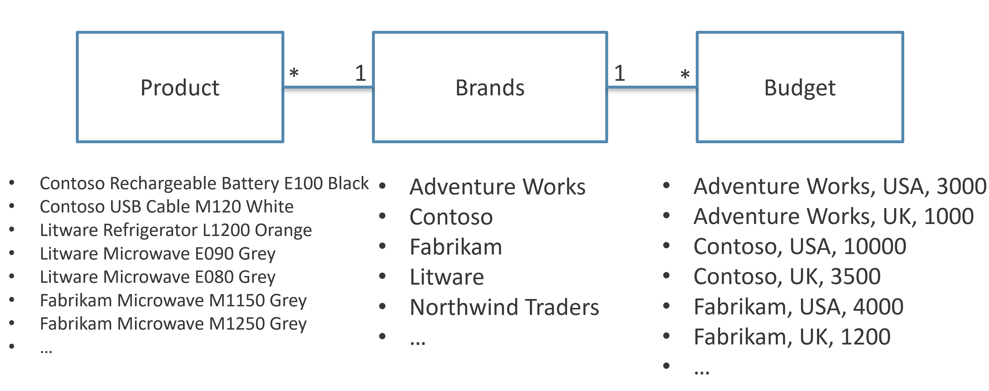
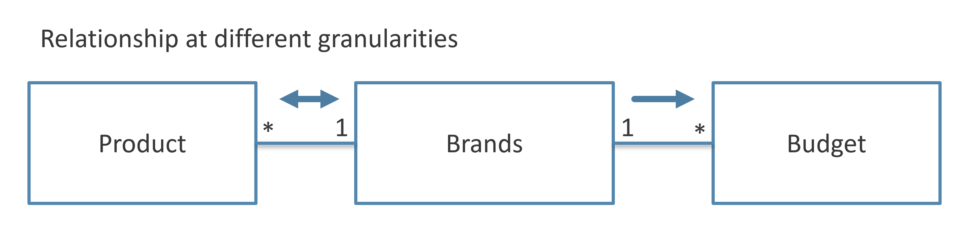
A logical relationship can exist between two tables whose granularity is not compatible with a physical SMR relationship. For example, consider the following model where the granularity of the Budget table is defined at the Customer[CountryRegion] and Product[Brand] level. The Customer table has one row for each customer, so there could be multiple rows with the same value for the CountryRegion column. Similarly, there is one row for each Product and several rows can have the same value for the Brand column.

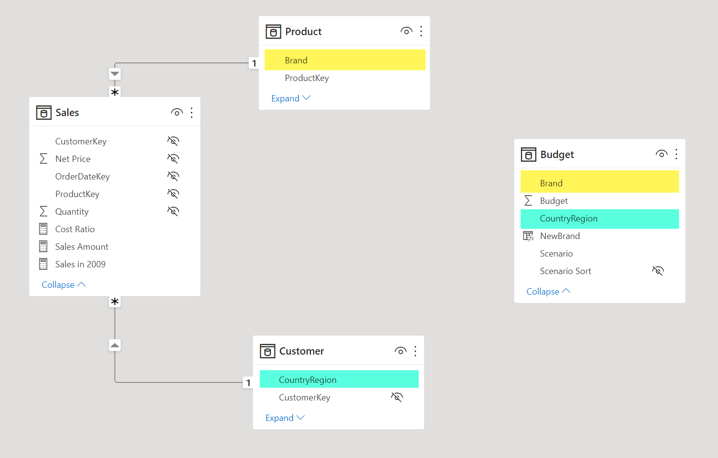
The cardinality of Product and Customer is the right one for the Sales table. In order to create a report that aggregates all the rows in Budget for a given product brand or customer country, one option is to apply two virtual relationships in a measure:

Budget Amount :=
CALCULATE (
    SUM ( Budget[Budget] ),
    TREATAS ( 
        VALUES ( 'Product'[Brand] ), 
        Budget[Brand] 
    ),
    TREATAS ( 
        VALUES ( Customer[CountryRegion] ), 
        Budget[CountryRegion] 
    )
)

However, any technique that transfers the filter using a virtual relationship implemented through a DAX expression might suffer a performance penalty compared to a solution based on physical relationships.

In order to use the more efficient SMR relationships, we can create a CountryRegions calculated table that contains all the values existing in either Customer[CountryRegion] or Budget[CountryRegion], and a Brands calculated table containing all the values existing in either Product[Brand] or Budget[Brand]:

CountryRegions =
DISTINCT (
    UNION (
        DISTINCT ( Customer[CountryRegion] ),
        DISTINCT ( Budget[CountryRegion] )
    )
)

Brands =
DISTINCT (
    UNION (
        DISTINCT ( Product[Brand] ),
        DISTINCT ( Budget[Brand] )
    )
)

The CountryRegions and Brands tables can be connected using simple SMR relationships to the Customer, Budget, and Product tables. By enabling the bidirectional filter on the relationship between Product and Brands, we materialize through two physical relationships the virtual relationship that transfers the filter from Product to Budget using the Brand column in both tables. In a similar way, Customer transfers the filter to Budget through the bidirectional filter between Customer and CountryRegions.

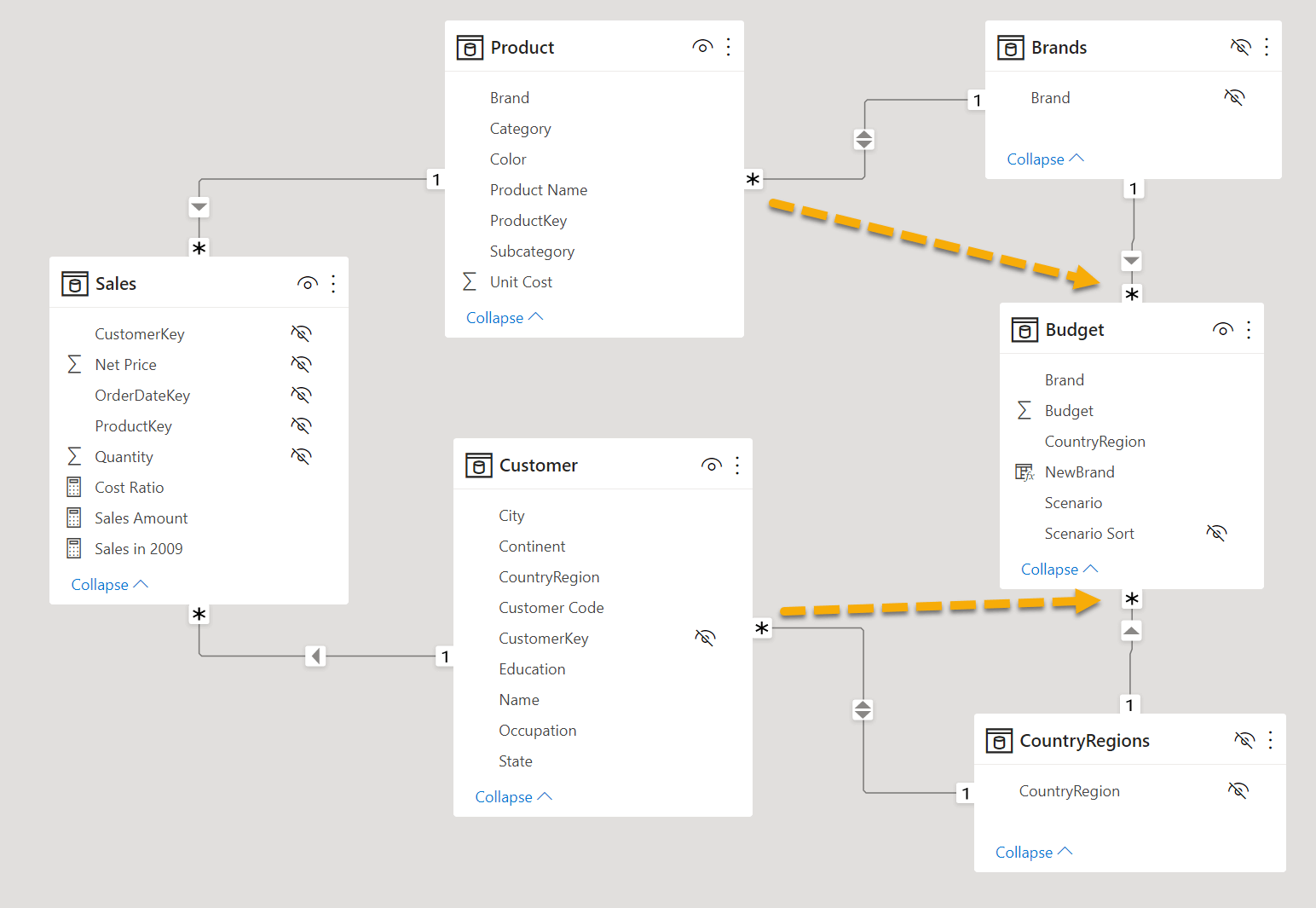
Although we recommend not to use bidirectional filters in a data model, this is one of the few cases where this practice is safe. Indeed, the calculated tables and two physical SMR relationships we created are just an artifact to implement a virtual relationship between two tables; the resulting virtual relationships transfer the filter in a single direction: Customer filters Budget and Product filters Budget. There are no ambiguities. It is also important to note that the Brands and CountryRegions calculated tables do not add any new information to the data model. They are simply a way to materialize a table whose cardinality allows the creation of two SMR relationships for each virtual relationship we need.

The following picture shows the granularity of the three tables involved in the virtual relationship between Product and Budget.

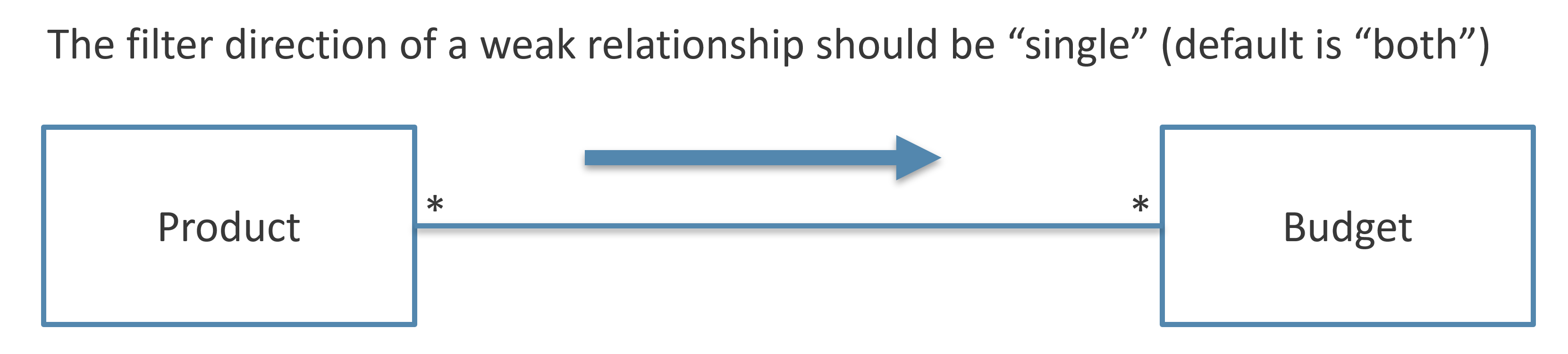
The virtual relationship between Product and Budget does not have a one-side. We can say that such a virtual relationship has a many-to-many cardinality. The artifact we just created can be obtained using an MMR relationship with a single filter, as shown in the following model.

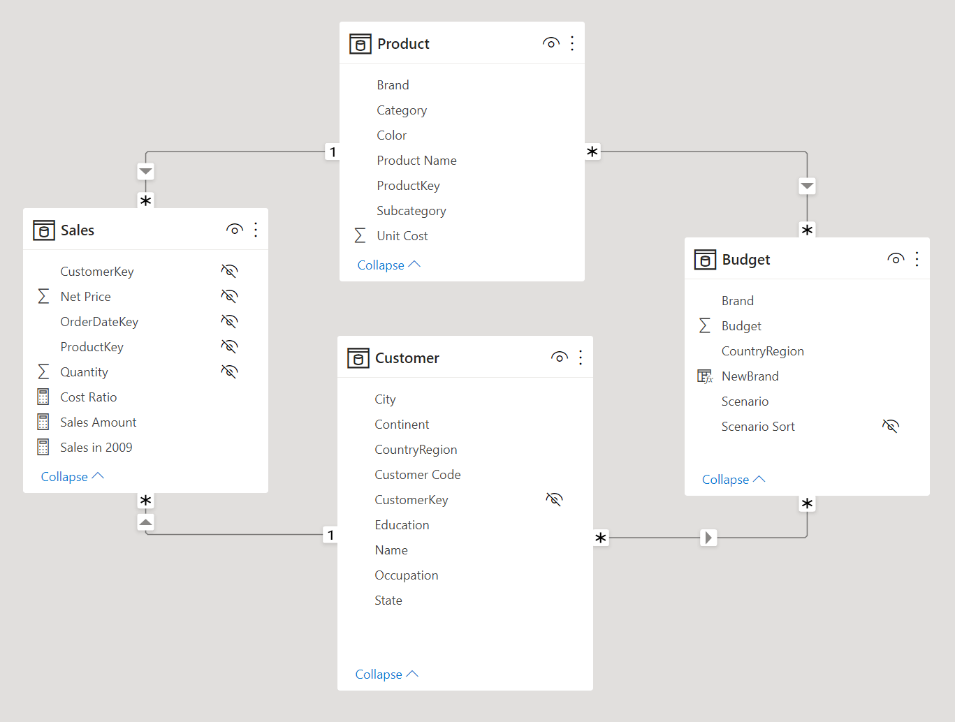
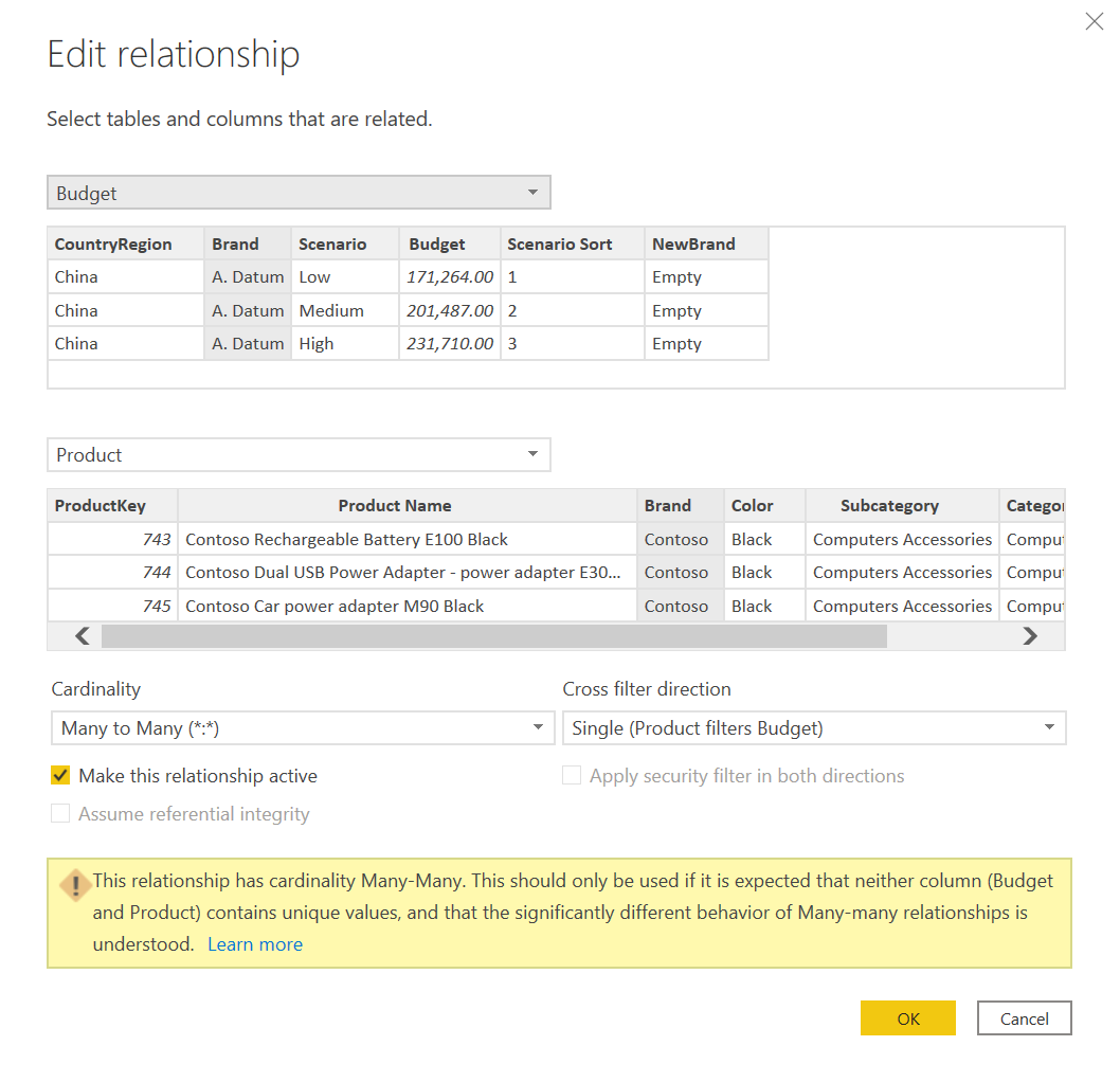
The relationship between Product and Budget must be defined with a many-to-many cardinality and a Single cross-filter direction. Power BI also displays a warning when you create an MMR relationship. It is important to keep the cross-filter direction as Single in order to avoid ambiguities in the data model.

Even though the MMR relationship is a single entity in the data model, its performance is not as good as the artifact that requires one calculated table and two SMR relationships. Indeed, there are no indexes created to support an MMR relationship in the storage engine. While an MMR relationship is faster than a virtual relationship implemented using TREATAS, it is not as good as an artifact based on two SMR relationships. The difference can be ignored when the cardinality of the column used in the relationship is in the range of 10 to 100 unique values. When there are thousands or more unique values in the column defining a relationship, you should consider creating the calculated table and the two SMR relationships instead of an MMR relationship.

Understanding different types of many-to-many relationships

The Tabular model allows users to create two different types of many-to-many relationships:

The many-to-many relationships between dimensions: these are the “classic” many-to-many relationships between dimensions in a dimensional model. These relationships require a bridge table containing data coming from the data source. The bridge table holds the information that defines the existing relationships between the entities. Without the bridge table, the relationships cannot be established.
The relationships at different granularities: these relationships use columns that do not correspond to the identity of the table, so the cardinality is “many” on both ends of the virtual relationship. A physical implementation of this type of relationship can use two SMR relationships connected to an intermediate table populated with the unique values of the column defining the relationship. The Tabular model enables users to create this relationship using an MMR relationship, which is always a limited relationship.

The “classic” many-to-many relationship is implemented using two SMR relationships in the order one-many/many-one. In order to implement a filter propagation from Customer to Account, the bidirectional filter must be enabled on the relationship connecting the Account table to the bridge table – AccountsCustomers in this example.

The relationship at different granularities is implemented using two SMR relationships in the order many-one/one-many, or by using a single MMR relationship in a Tabular model. In both cases, the virtual relationship should propagate the filter in a single direction. If the relationship is implemented using two SMR relationships, in order to propagate the filter from Product to Budget, the bidirectional filter must be enabled on the relationship connecting the Product table to the intermediate table – Brands in this example.

A single MMR relationship can simplify the creation of a relationship at different granularities. It is considered best practice to specify the correct direction of the relationship, which should be Single. By default, Power BI creates these relationships with a bidirectional filter propagation, which can create ambiguities in the data model.

Conclusions

There are different ways to implement a logical relationship in a Tabular model. DAX provides flexible techniques to implement any kind of virtual relationship between entities, but only physical relationships in the data model provide the best results in terms of performance. Filter propagation direction and granularity of the relationships are key concepts to create the proper physical implementation of a logical relationship.

The classic notion of “many-to-many” relationships in Dimensional modeling does not correspond to what is referred to as a “many-to-many cardinality relationship” in a Tabular model. The latter is just an alternative to an artifact – based on two physical relationships and a calculated table – that enables users to define a relationship between entities with a granularity different from the granularity of the tables. For this reason, when referring to a Tabular model it is better to use the acronyms SMR and MMR to identify Single-Many-Relationship and Many-Many-Relationship, respectively. The term “many-to-many” relationship should only be used to describe the logical relationship between dimensions, which is implemented through two SMR relationships in the physical model.