Standard time-related calculations

In this pattern, we show you how to compute time-related calculations, like year-to-date, same period last year, and percentage growth using a standard calendar. The great advantage of working with a standard calendar is that you can rely on several built-in time intelligence functions. The built-in functions are designed in such a way that they provide the correct result for the most common requirements.
In case your requirement cannot be fulfilled by the built-in functions, or if you have a non-standard calendar, then you should use regular (non-time-related) DAX functions to reach the same goal. This way, you customize the result of your code at will. That said, if you need custom calculations, then you also need to enrich your date table with a set of columns that are needed by the DAX formulas to move the filter. These custom calculations are covered in the Custom time-related calculations pattern.
If you are using a regular Gregorian calendar, then the formulas in this pattern are the easiest and most effective way of producing time intelligence calculations. Keep in mind that standard DAX time intelligence functions only support a regular Gregorian calendar – that is a calendar with 12 months, each month with its Gregorian number of days, quarters made up of three months, and all the regular aspects of a calendar that we are used to.
Introduction to time intelligence calculations
In order to use any time intelligence calculation, you need a well-formed date table. The Date table must satisfy the following requirements:
- All dates need to be present for the years required. The Date table must always start on January 1 and end on December 31, including all the days in this range. If the report only references fiscal years, then the date table must include all the dates from the first to the last day of a fiscal year. For example, if the fiscal year 2008 starts on July 1, 2007, then the Date table must include all the days from July 1, 2007 to June 30, 2008.
- There needs to be a column with a DateTime or Date data type containing unique values. This column is usually called Date. Even though the Date column is often used to define relationships with other tables, this is not required. Still, the Date column must contain unique values and should be referenced by the Mark as Date Table feature. In case the column also contains a time part, no time should be used – for example, the time should always be 12:00 am.
- The Date table must be marked as a date table in the model, in case the relationship between the Date table and any other table (like Sales in our example) is not based on the Date
There are several ways to build a Date table. The way you build the Date table does not affect how you use the standard time intelligence calculations, as long as the date table satisfies the requirements. If you already have a Date table that works well for your report, just import it and mark it as a date table after having checked that it satisfies the minimum requirements. If you do not have a Date table, you can create one using a DAX calculated table as described later.
It is a best practice to apply the Mark as a Date Table setting to the Date table used for time intelligence calculations. The Mark as a Date Table setting adds a REMOVEFILTERS modifier over the Date table every time a filter is applied to the Date column. This action (applying a filter on the Date column) is performed by all the time intelligence functions used in CALCULATE. DAX implements the same behavior if you define the relationship between Sales and Date using the Date column. Nevertheless, applying the Mark as a Date Table setting to a date table is a best practice. If you have multiple date tables, you can mark all of them as date tables.
If you do not use the Mark as a Date Table setting and you do not use the date column for the relationship, then you must add a REMOVEFILTERS over the Date table whenever you use a time intelligence function in CALCULATE. This behavior is described in more detail in the article Time Intelligence in Power BI Desktop.
What are standard DAX time intelligence functions
The standard time intelligence functions are table functions returning a list of dates used as a filter in CALCULATE. The result of a time intelligence function can be obtained by writing a more complex filter expression. For example, the DATESYTD function returns all the dates in the same year between the first day of the year and the last day visible in the filter context. The following expression:
DATESYTD ( 'Date'[Date] )
corresponds to the following FILTER expression:
VAR LastDateAvailable = MAX ( 'Date'[Date] )
VAR FirstJanuaryOfLastDate = DATE ( YEAR ( LastDateAvailable ), 1, 1 )
RETURN
    FILTER (
        ALL ( 'Date'[Date] ),
        AND (
            'Date'[Date] >= FirstJanuaryOfLastDate,
            'Date'[Date] <= LastDateAvailable
        )
    )
There are many time intelligence functions, most of which we present in this pattern. Be mindful: time intelligence functions should be used as filter arguments of CALCULATE, and sometimes you will resort to variables to achieve that. It is dangerous to use time intelligence functions in iterators, because of the implicit context transition that is triggered to retrieve the dates active from the filter context. More details about this behavior are available in the DAX Guide documentation, like https://dax.guide/datesytd/ .
The following is a quick guide to the best practices when using time intelligence functions:
- Use time intelligence functions like DATESYTD only in filter arguments of CALCULATE / CALCULATETABLE, or to assign filters to variables.
- Use scalar functions like EDATE and EOMONTH in DAX formulas returning a value – also known as scalar expressions. These functions are not time intelligence functions and can be used in expressions evaluated in a row context.
- Use CONVERT to convert a date into a number and vice versa.
- A complete updated list of time intelligence functions is available at https://dax.guide/.
DAX beginners often confuse time intelligence functions with regular – scalar – time functions. This confusion leads to common mistakes that can be avoided by following these suggestions:
- DO NOT use DATEADD to return the previous or the following day. You can use simple mathematical operators to do that.
- DO NOT use PREVIOUSDAY to compute the previous day in a scalar expression. You can just subtract one from a date to obtain the previous day in a scalar expression.
- DO NOT use EOMONTH as a filter – use ENDOFMONTH instead. EOMONTH is a scalar expression. ENDOFMONTH is a time intelligence function. Always pay attention to the return type of a function: only table functions are time intelligence functions, and they should not be used in scalar expressions.
Disabling the Auto Date/Time
Power BI can automatically add a Date table to a data model. Yet, we strongly suggest disabling the automatic Date table created by Power BI and importing or creating an explicit Date table instead. More details are included in the article Automatic time intelligence in Power BI.
The presence of an automatic Date table also enables a specific syntax called column variation. Column variations are expressed with a dot after the date column, followed by a column of the date table that is created automatically:
Sales[Order Date].[Date]
Power BI quick measures make extensive use of column variations when used over an automatic Date table. We do not rely on the date tables created automatically in Power BI because we want to maintain maximum flexibility and maximum control over our model. The syntax of column variations is not used for Date tables that are part of the model and thus are not created automatically.
Limitations of standard time intelligence functions
The standard time intelligence functions work on a regular Gregorian calendar. They have several limitations, listed in this section. When your requirements are not compatible with these limitations, you need another pattern (see Custom time-related calculations and Week-related calculations).
- The year starts on the first of January. There is limited support for fiscal calendars starting at a different date. However, the first day of the fiscal year must always be the same for every year and cannot be the first of March, because of historical bugs related to leap years.
- The quarters always start on the first of January, April, July, and October. The range of a quarter cannot be modified.
- A month is always a calendar month.
- Filters of additional columns such as Day of Week or Working Day might not be supported correctly by standard time intelligence functions. More details about possible workarounds are available in the section, “Filtering other date attributes”.
Consequently, many advanced calculations like calculations over weeks are not supported by the standard time intelligence calculations. These advanced calculations require a custom calendar.
Building a Date table
DAX time intelligence functions work on any standard Gregorian calendar table. If you already have a Date table, you can import the table and use it without any issue. If a Date table is not available, you can create one using a DAX calculated table. As an example, the following DAX expression defines the simple Date table used in this chapter:
Date =
VAR FirstFiscalMonth = 7  -- First month of the fiscal year
VAR FirstDayOfWeek = 0    -- 0 = Sunday, 1 = Monday, ...
VAR FirstYear =           -- Customizes the first year to use
    YEAR ( MIN ( Sales[Order Date]  ))
RETURN
GENERATE (
    FILTER (
        CALENDARAUTO (),
        YEAR ( [Date] ) >= FirstYear
    ),
    VAR Yr = YEAR ( [Date] )             -- Year Number
    VAR Mn = MONTH ( [Date] )            -- Month Number (1-12)
    VAR Qr = QUARTER ( [Date] )          -- Quarter Number (1-4)
    VAR MnQ = Mn - 3 * (Qr - 1)          -- Month in Quarter (1-3)
    VAR Wd = WEEKDAY ( [Date], 1 ) - 1   -- Weekday Number (0 = Sunday, 1 = Monday, ...)
    VAR Fyr =                            -- Fiscal Year Number
        Yr + 1 * ( FirstFiscalMonth > 1 && Mn >= FirstFiscalMonth )
    VAR Fqr =                            -- Fiscal Quarter (string)
        FORMAT ( EOMONTH ( [Date], 1 - FirstFiscalMonth ), "\QQ" )
    RETURN ROW (
        "Year", DATE ( Yr, 12, 31 ),
        "Year Quarter", FORMAT ( [Date], "\QQ-YYYY" ),
        "Year Quarter Date", EOMONTH ( [Date], 3 - MnQ ),
        "Quarter", FORMAT ( [Date], "\QQ" ),
        -- "Year Month", EOMONTH ( [Date], 0 ), -- use this for end-of-month
        "Year Month", EOMONTH ( [Date], -1 ) + 1, -- use this for beginning-of-month
        "Month", DATE ( 1900, MONTH ( [Date] ), 1 ),
        "Day of Week", DATE ( 1900, 1, 7 + Wd + (7 * (Wd < FirstDayOfWeek)) ),
        "Fiscal Year", DATE ( Fyr + (FirstFiscalMonth = 1), FirstFiscalMonth, 1 ) - 1,
        "Fiscal Year Quarter", "F" & Fqr & "-" & Fyr,
        "Fiscal Year Quarter Date", EOMONTH ( [Date], 3 - MnQ ),
        "Fiscal Quarter", "F" & Fqr
    )
)
Using beginning-of-month instead of end-of-month could be better for month-based charts in Power BI. More details in the Creating a simpler and chart-friendly Date table in Power BI article.
You can customize the first three variables to build a Date table that meets specific business requirements. In order to obtain the correct result, the columns must be configured in the data model as follows – when the column is not text, it is a Date data type with standard or custom format:
- Date: m/dd/yyyy (8/14/2007), used as a column to mark as date table
- Year: yyyy (2007)
- Year Quarter: Text (Q3-2008)
- Year Quarter Date: Hidden (9/30/2008)
- Quarter: Text (Q1)
- Year Month: mmm yyyy (Aug 2007)
- Month: mmm (Aug)
- Day of Week: ddd (Tue)
- Fiscal Year: \F\Y yyyy (FY 2008)
- Fiscal Year Quarter: Text (FQ1-2008)
- Fiscal Year Quarter Date: Hidden (9/30/2008)
- Fiscal Quarter: Text (FQ1)
The Date table in this pattern has two hierarchies:
- Calendar: Year (Year), Quarter (Year Quarter), Month (Year Month)
- Fiscal: Year (Fiscal Year), Quarter (Fiscal Year Quarter), Month (Year Month)
Regardless of the source, the Date table must also include a hidden DateWithSales calculated column to use the formulas of this pattern:
DateWithSales =
'Date'[Date] <= MAX ( Sales[Order Date] )
The Date[DateWithSales] column is TRUE if the date is on or before the last date with transactions in the Sales table; it is FALSE otherwise. In other words, DateWithSales is TRUE for “past” dates and FALSE for “future” dates, where “past” and “future” are relative to the last date with transactions in Sales.
Controlling the visualization in future dates
Most of the time intelligence calculations should not display values for dates after the last date available. For example, a year-to-date calculation can also show values for future dates, but we want to hide those values. The dataset used in these examples ends on August 15, 2009. Therefore, we consider the month of August 2009, the third quarter of 2009 (Q3-2009), and the year 2009 as the last periods with data. Any date later than August 15, 2019 is considered as future, and we want to hide values there.
In order to avoid showing results in future dates, we use the following ShowValueForDates measure. ShowValueForDates returns TRUE if the time period selected is not after the last period with data:
ShowValueForDates :=
VAR LastDateWithData =
    CALCULATE (
        MAX ( 'Sales'[Order Date] ),
        REMOVEFILTERS ()
    )
VAR FirstDateVisible =
    MIN ( 'Date'[Date] )
VAR Result =
    FirstDateVisible <= LastDateWithData
RETURN
    Result
The ShowValueForDates measure is hidden. It is a technical measure created to reuse the same logic in many different time-related calculations, and the user should not use ShowValueForDates directly in a report.
Naming convention
This section describes the naming convention we adopted to reference the time intelligence calculations. A simple categorization shows whether a calculation:
- shifts over a period of time, for example the same period in the previous year;
- performs an aggregation, for example year-to-date; or
- compares two time periods, for example this year compared to last year.
| Acronym | Description | Shift | Aggregation | Comparison |
| YTD | Year-to-date | |||
| QTD | Quarter-to-date | |||
| MTD | Month-to-date | |||
| MAT | Moving annual total | |||
| PY | Previous year | |||
| PQ | Previous quarter | |||
| PM | Previous month | |||
| PYC | Previous year complete | |||
| PQC | Previous quarter complete | |||
| PMC | Previous month complete | |||
| PP | Previous period (automatically selects year, quarter, or month) | |||
| PYMAT | Previous year moving annual total | |||
| YOY | Year-over-year | |||
| QOQ | Quarter-over-quarter | |||
| MOM | Month-over-month | |||
| MATG | Moving annual total growth | |||
| POP | Period-over-period (automatically selects year, quarter, or month) | |||
| PYTD | Previous year-to-date | |||
| PQTD | Previous quarter-to-date | |||
| PMTD | Previous month-to-date | |||
| YOYTD | Year-over-year-to-date | |||
| QOQTD | Quarter-over-quarter-to-date | |||
| MOMTD | Month-over-month-to-date | |||
| YTDOPY | Year- to-date-over-previous-year | |||
| QTDOPQ | Quarter-to-date-over-previous-quarter | |||
| MTDOPM | Month-to-date-over-previous-month |
Computing period-to-date totals
The year-to-date, quarter-to-date, and month-to-date calculations modify the filter context for the Date table, applying a range of dates as a filter that overwrites the filter for the period selected.
All these calculations can be implemented using a regular CALCULATE with a time intelligence function, or with one of the TOTAL functions such as TOTALYTD. TOTAL functions are just syntactic sugar for the CALCULATE version. We show them as a reference, even though we prefer the CALCULATE version – indeed, using CALCULATE makes the formula logic more evident, and it provides more flexibility than TOTAL functions do. The formulas using the TOTAL functions are marked as (2) in the following examples. The purpose of showing them is only to show that they return the same values as the CALCULATE version does.
Year-to-date total
The year-to-date aggregates data starting on January 1 of the year, as shown in Figure 1.
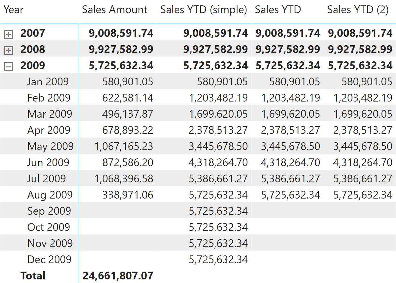
The year-to-date total of a measure can rely on the DATESYTD function this way:
Sales YTD (simple) :=
CALCULATE (
    [Sales Amount],
    DATESYTD ( 'Date'[Date] )
)
DATESYTD returns the set of dates from the first day of the current year, up to the last date visible in the filter context. Therefore, the Sales YTD (simple) measure shows data even for future dates in the year. We can avoid this behavior in the Sales YTD measure by returning a result only when the ShowValueForDates measure returns TRUE:
Sales YTD :=
IF (
    [ShowValueForDates],
    CALCULATE (
        [Sales Amount],
        DATESYTD ( 'Date'[Date] )
    )
)
If the report is based on a fiscal year that does not correspond to the calendar year, DATESYTD requires an additional argument to identify the last day of the fiscal year. Take for example, the report in Figure 2.
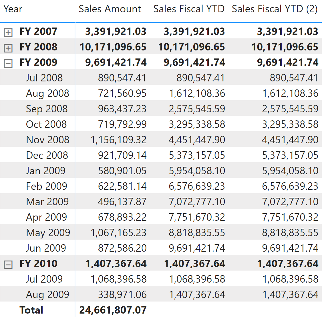
The Sales Fiscal YTD measure specifies the last day and month of the fiscal year in the second argument of DATESYTD. The following measure uses June 30 as the last day of the fiscal year. The second argument of DATESYTD must be a constant value (also called a literal) corresponding to the definition of the fiscal year in the Date table; it cannot be computed dynamically:
Sales Fiscal YTD :=
IF (
    [ShowValueForDates],
    CALCULATE (
        [Sales Amount],
        DATESYTD ( 'Date'[Date], "6-30" )
    )
)
The TOTALYTD function is a possible alternative to DATESYTD:
Sales YTD (2) :=
IF (
    [ShowValueForDates],
    TOTALYTD (
        [Sales Amount],
        'Date'[Date]
    )
)
Sales Fiscal YTD (2) :=
IF (
    [ShowValueForDates],
    TOTALYTD (
        [Sales Amount],
        'Date'[Date],
        "6-30"
    )
)
Quarter-to-date total
The quarter to date aggregates data from the first day of the quarter, as shown in Figure 3.
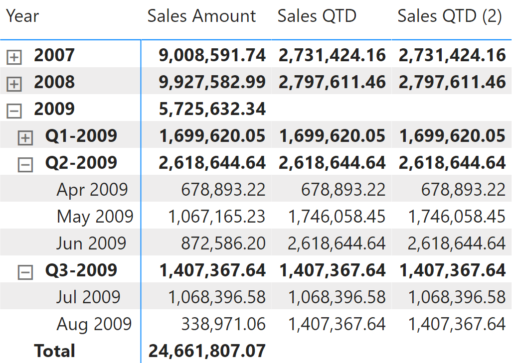
The quarter-to-date total of a measure is computed with the DATESQTD function as follows:
Sales QTD :=
IF (
    [ShowValueForDates],
    CALCULATE (
        [Sales Amount],
        DATESQTD ( 'Date'[Date] )
    )
)
The TOTALQTD is a possible alternative to DATESQTD:
Sales QTD (2) :=
IF (
    [ShowValueForDates],
    TOTALQTD (
        [Sales Amount],
        'Date'[Date]
    )
)
Month-to-date total
The month to date aggregates data from the first day of the month, as shown in Figure 4.
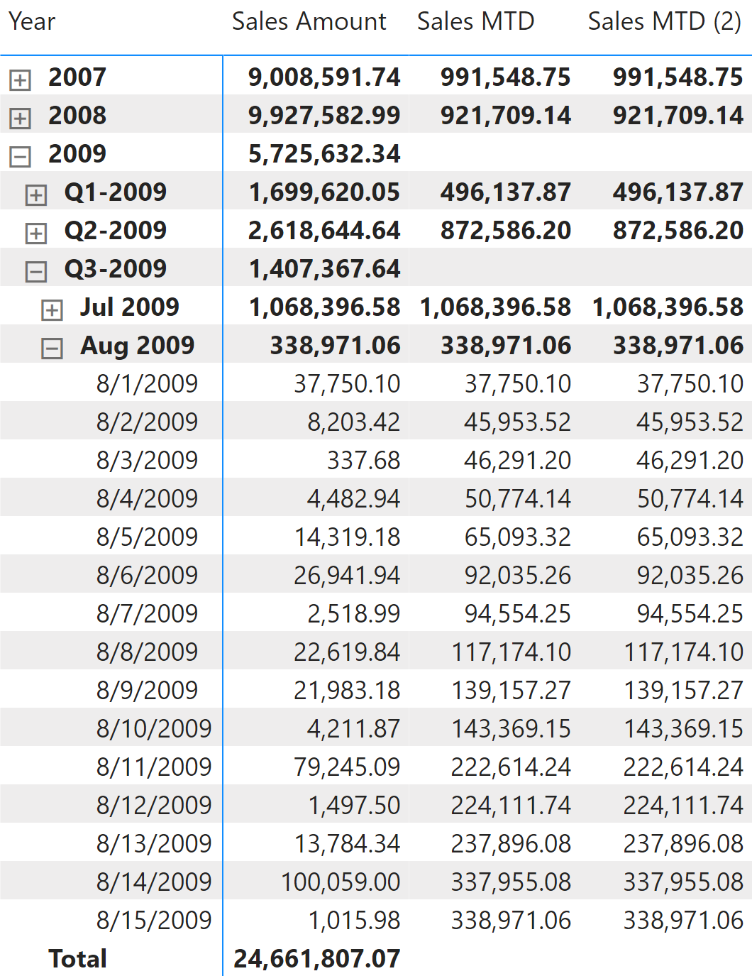
The month-to-date total of a measure is computed with the DATESMTD function this way:
Sales MTD :=
IF (
    [ShowValueForDates],
    CALCULATE (
        [Sales Amount],
        DATESMTD ( 'Date'[Date] )
    )
)
The TOTALMTD is a possible alternative to DATESMTD :
Sales MTD (2) :=
IF (
    [ShowValueForDates],
    TOTALMTD (
        [Sales Amount],
        'Date'[Date]
    )
)
Computing period-over-period growth
A common requirement is to compare a time period with the same time period in the previous year, quarter, or month. The last month/quarter/year could be incomplete; so in order to achieve a fair comparison, the comparison should consider an equivalent period. For these reasons, the calculations shown in this section use the Date[DateWithSales] calculated column, as described in the article Hiding future dates for calculations in DAX.
Year-over-year growth
Year-over-year compares a period to the equivalent period in the previous year. In this example, data is available until August 15, 2009. For this reason, Sales PY shows numbers related to 2008 only considering transactions prior to August 15, 2008. Figure 5 shows that Sales Amount of August 2008 is 721,560.95, whereas Sales PY for August 2009 returns 296,529.51 because the measure only considers sales up to August 15, 2008.
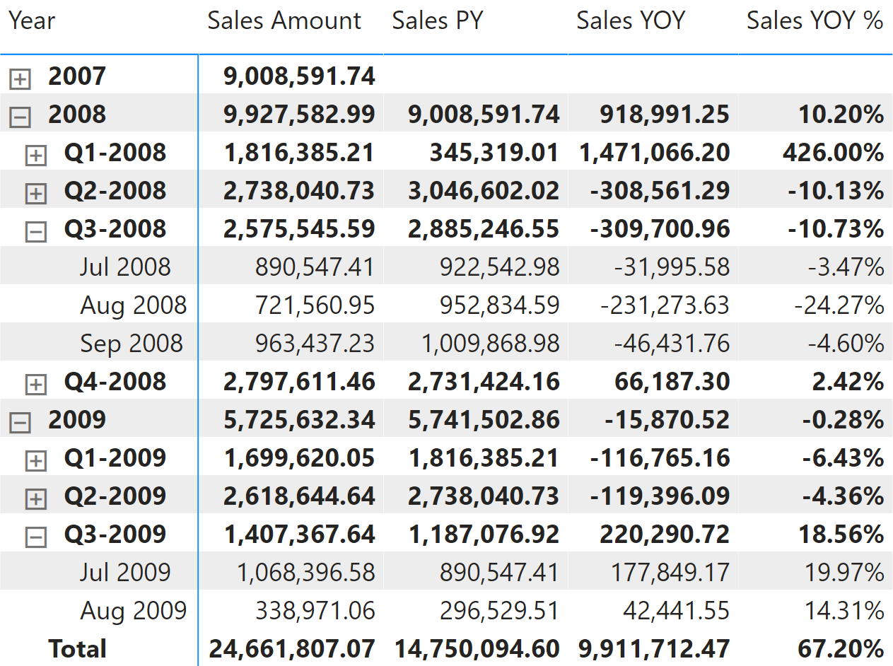
Sales PY uses DATEADD and filters Date[DateWithSales] to guarantee a fair comparison of the last period with data. The year-over-year growth is computed as an amount in Sales YOY, and as a percentage in Sales YOY %. Both measures use Sales PY to only consider dates up to August 15, 2009:
Sales PY :=
IF (
    [ShowValueForDates],
    CALCULATE (
        [Sales Amount],
        CALCULATETABLE (
            DATEADD ( 'Date'[Date], -1, YEAR ),
            'Date'[DateWithSales] = TRUE
        )
    )
)
Sales YOY :=
VAR ValueCurrentPeriod = [Sales Amount]
VAR ValuePreviousPeriod = [Sales PY]
VAR Result =
    IF (
        NOT ISBLANK ( ValueCurrentPeriod ) && NOT ISBLANK ( ValuePreviousPeriod ),
        ValueCurrentPeriod - ValuePreviousPeriod
    )
RETURN
    Result
Sales YOY % :=
DIVIDE (
    [Sales YOY],
    [Sales PY]
)
Sales PY can also be written using SAMEPERIODLASTYEAR. SAMEPERIODLASTYEAR is easier to read, but it does not offer any performance benefit. This is because internally, it is translated into the DATEADD function used in previous formulas:
Sales PY (2) :=
IF (
    [ShowValueForDates],
    CALCULATE (
        [Sales Amount],
        CALCULATETABLE (
            SAMEPERIODLASTYEAR ( 'Date'[Date] ),
            'Date'[DateWithSales] = TRUE
        )
    )
)
Quarter-over-quarter growth
Quarter-over-quarter compares a period with the equivalent period in the previous quarter. In this example, data is available until August 15, 2009, which is the first half of the third quarter of 2009. Therefore, Sales PQ for August 2009 (the second month of the third quarter) shows sales until May 15, 2009, which is the first half of the second month of the previous quarter. Figure 6 shows that Sales Amount of May 2009 is 1,067,165.23, whereas Sales PQ for August 2009 returns 435,306.10, only taking into account sales made prior to May 15, 2009.
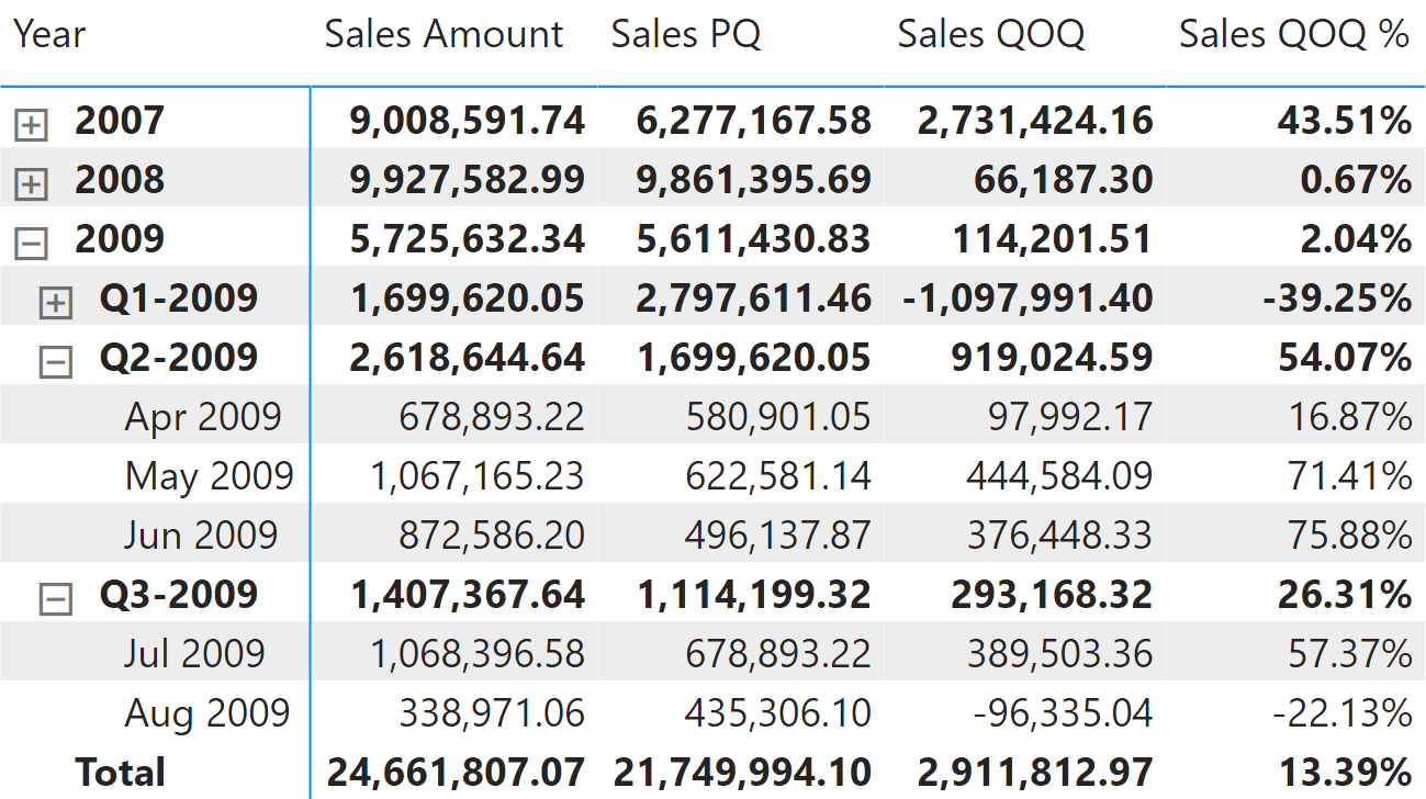
Sales PQ uses DATEADD and filters Date[DateWithSales] to guarantee a fair comparison with the last period with data. The quarter-over-quarter growth is computed as an amount in Sales QOQ and as a percentage in Sales QOQ %. Both measures use Sales PQ to guarantee the same fair comparison:
Sales PQ :=
IF (
    [ShowValueForDates],
    CALCULATE (
        [Sales Amount],
        CALCULATETABLE (
            DATEADD ( 'Date'[Date], -1, QUARTER ),
            'Date'[DateWithSales] = TRUE
        )
    )
)
Sales QOQ :=
VAR ValueCurrentPeriod = [Sales Amount]
VAR ValuePreviousPeriod = [Sales PQ]
VAR Result =
    IF (
        NOT ISBLANK ( ValueCurrentPeriod ) && NOT ISBLANK ( ValuePreviousPeriod ),
        ValueCurrentPeriod - ValuePreviousPeriod
    )
RETURN
    Result
Sales QOQ % :=
DIVIDE (
    [Sales QOQ],
    [Sales PQ]
)
Month-over-month growth
Month-over-month compares a time period with its equivalent in the previous month. In this example, data is only available until August 15, 2009. For this reason, Sales PM only considers sales between July 1-15, 2009 in order to return a value for August 2009. That way, it only returns the corresponding portion of the previous month. Figure 7 shows that Sales Amount for July 2009 is 1,068,396.58, whereas Sales PM of August 2019 returns 584,212.78, since it only takes into account sales prior to July 15, 2009.
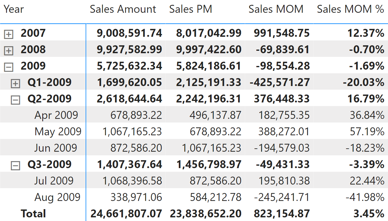
Sales PM uses DATEADD and filters the Date[DateWithSales] column to guarantee a fair comparison of the last period with data. The month-over-month growth is computed as an amount in Sales MOM and as a percentage in Sales MOM %. Both measures use Sales PM to guarantee the same fair comparison:
Sales PM :=
IF (
    [ShowValueForDates],
    CALCULATE (
        [Sales Amount],
        CALCULATETABLE (
            DATEADD ( 'Date'[Date], -1, MONTH ),
            'Date'[DateWithSales] = TRUE
        )
    )
)
Sales MOM :=
VAR ValueCurrentPeriod = [Sales Amount]
VAR ValuePreviousPeriod = [Sales PM]
VAR Result =
    IF (
        NOT ISBLANK ( ValueCurrentPeriod )
            && NOT ISBLANK ( ValuePreviousPeriod ),
        ValueCurrentPeriod - ValuePreviousPeriod
    )
RETURN
    Result
Sales MOM % :=
DIVIDE (
    [Sales MOM],
    [Sales PM]
)
Period-over-period growth
Period-over-period growth automatically selects one of the measures previously described in this section based on the current selection of the visualization. For example, it returns the value of month-over-month growth measures if the visualization displays data at the month level, switching to year-over-year growth measures if the visualization shows the total at the year level. The expected result is visible in Figure 8.
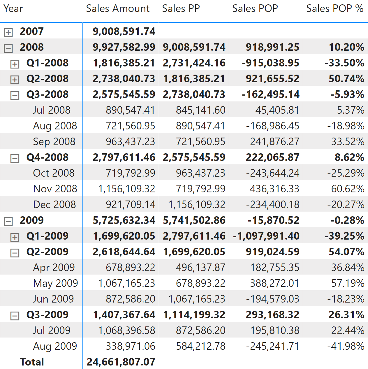
The three measures Sales PP, Sales POP, and Sales POP % redirect the evaluation to the corresponding year, quarter, and month measures depending on the level selected in the report. The ISINSCOPE function detects the level used in the report. The arguments passed to ISINSCOPE are the attributes used in the rows of the Matrix visual in Figure 8. The measures are defined as follows:
Sales POP % :=
SWITCH (
    TRUE,
    ISINSCOPE ( 'Date'[Year Month] ), [Sales MOM %],
    ISINSCOPE ( 'Date'[Year Quarter] ), [Sales QOQ %],
    ISINSCOPE ( 'Date'[Year] ), [Sales YOY %]
)
Sales POP :=
SWITCH (
    TRUE,
    ISINSCOPE ( 'Date'[Year Month] ), [Sales MOM],
    ISINSCOPE ( 'Date'[Year Quarter] ), [Sales QOQ],
    ISINSCOPE ( 'Date'[Year] ), [Sales YOY]
)
Sales PP :=
SWITCH (
    TRUE,
    ISINSCOPE ( 'Date'[Year Month] ), [Sales PM],
    ISINSCOPE ( 'Date'[Year Quarter] ), [Sales PQ],
    ISINSCOPE ( 'Date'[Year] ), [Sales PY]
)
Computing period-to-date growth
The growth of a “to-date” measure is the comparison of the “to-date” measure with the same measure over an equivalent period with a specific offset. For example, you can compare a year-to-date aggregation against the year-to-date in the previous year, that is with an offset of one year.
All the measures in this set of calculations take care of partial periods. Because data is available only until August 15, 2009 in our example, the measures make sure that data in the previous year does not consider dates after August 15, 2019.
Year-over-year-to-date growth
Year-over-year-to-date growth compares the year-to-date at a specific date with the year-to-date at an equivalent date in the previous year. Figure 9 shows that Sales PYTD in 2009 is only considering transactions until August 15, 2008. For this reason, Sales YTD of Q3-2008 is 7,129,971.53, whereas Sales PYTD for Q3-2009 is less: 5,741,502.86.
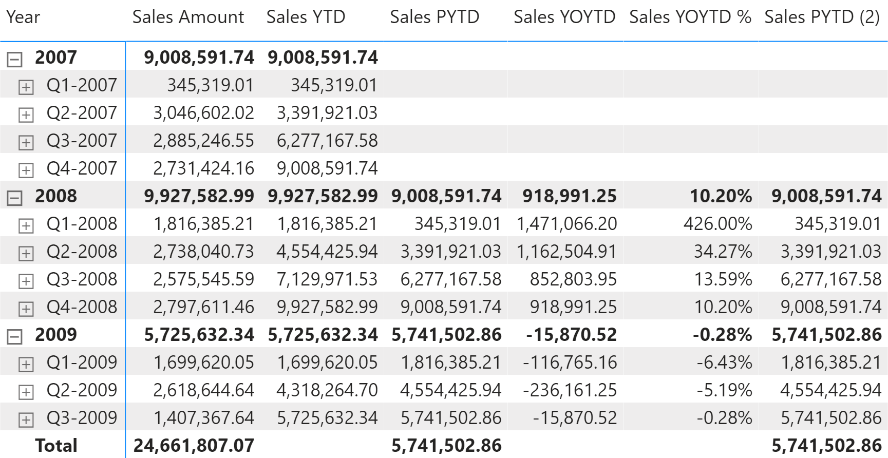
Sales PYTD uses DATEADD and filters the Date[DateWithSales] column to guarantee a fair comparison of the last period with data. Sales YOYTD and Sales YOYTD % rely on Sales PYTD to guarantee the same fair comparison:
Sales PYTD :=
IF (
    [ShowValueForDates],
    CALCULATE (
        [Sales YTD],
        CALCULATETABLE (
            DATEADD ( 'Date'[Date], -1, YEAR ),
            'Date'[DateWithSales] = TRUE
        )
    )
)
Sales YOYTD :=
VAR ValueCurrentPeriod = [Sales YTD]
VAR ValuePreviousPeriod = [Sales PYTD]
VAR Result =
    IF (
        NOT ISBLANK ( ValueCurrentPeriod )
            && NOT ISBLANK ( ValuePreviousPeriod ),
        ValueCurrentPeriod - ValuePreviousPeriod
    )
RETURN
    Result
Sales YOYTD % :=
DIVIDE (
    [Sales YOYTD],
    [Sales PYTD]
)
Sales PYTD shifts the date filter back one year by using DATEADD. Using DATEADD makes it easy to apply shifts of two or more years. However, to shift dates back by one year Sales PYTD can also be written using SAMEPERIODLASTYEAR as in the following example, which internally uses DATEADD as in the previous example:
Sales PYTD (2) :=
IF (
    [ShowValueForDates],
    CALCULATE (
        [Sales YTD],
        CALCULATETABLE (
            SAMEPERIODLASTYEAR ( 'Date'[Date] ),
            'Date'[DateWithSales] = TRUE
        )
    )
)
Quarter-over-quarter-to-date growth
Quarter-over-quarter-to-date growth compares the quarter-to-date at a specific date with the quarter-to-date at an equivalent date in the previous quarter. Figure 10 shows that Sales PQ in August 2009 is only considering transactions until May 15, 2009, to only get the first half of the previous quarter. For this reason Sales QTD of May 2009 is 1,746,058.45, whereas Sales PQTD for August 2009 is lower: 1,114,199.32.
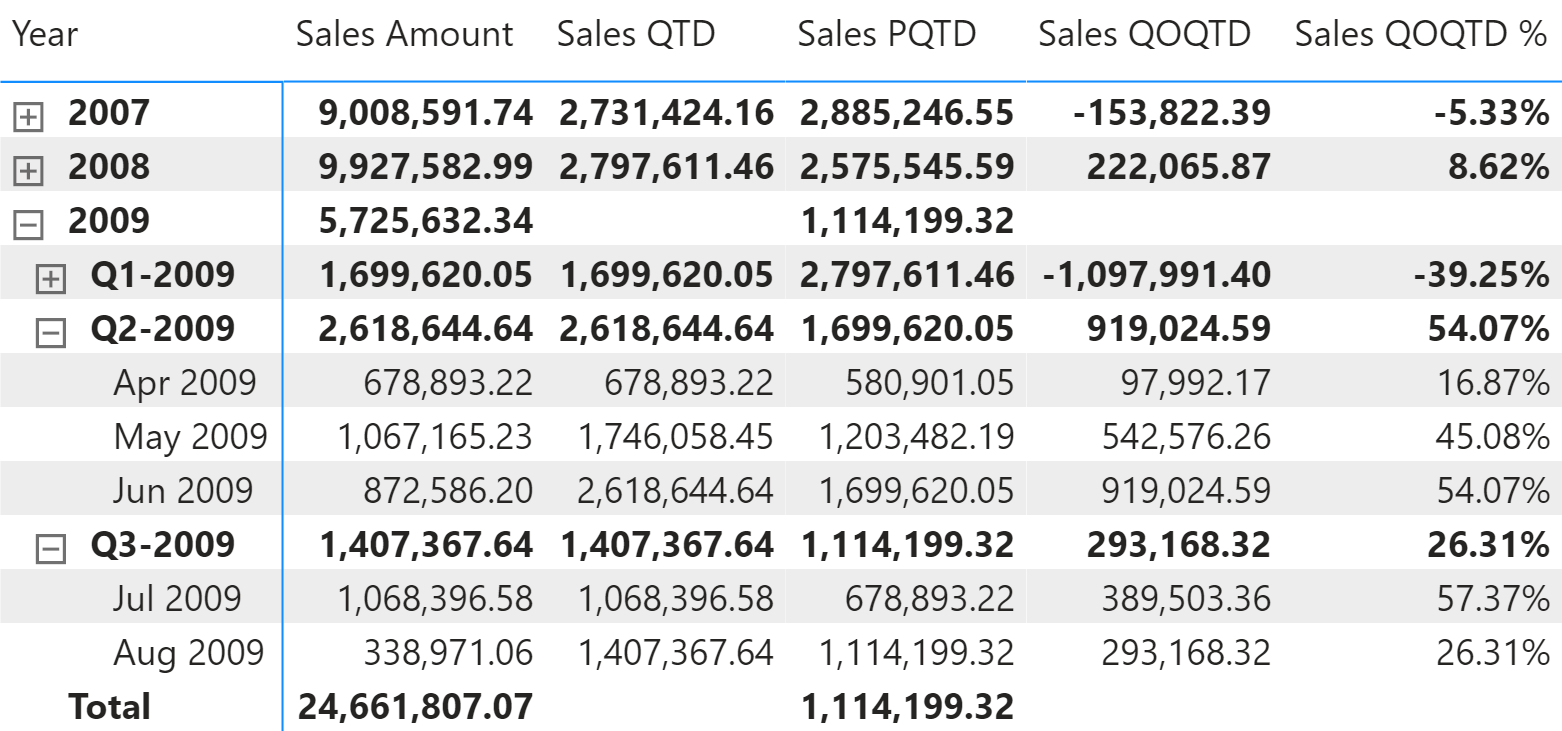
Sales PQTD uses DATEADD and filters the Date[DateWithSales] column to guarantee a fair comparison of the last period with data. Sales QOQTD and Sales QOQTD % rely on Sales PQTD to guarantee the same fair comparison:
Sales PQTD :=
IF (
    [ShowValueForDates],
    CALCULATE (
        [Sales QTD],
        CALCULATETABLE (
            DATEADD ( 'Date'[Date], -1, QUARTER ),
            'Date'[DateWithSales] = TRUE
        )
    )
)
Sales QOQTD :=
VAR ValueCurrentPeriod = [Sales QTD]
VAR ValuePreviousPeriod = [Sales PQTD]
VAR Result =
    IF (
        NOT ISBLANK ( ValueCurrentPeriod )
            && NOT ISBLANK ( ValuePreviousPeriod ),
        ValueCurrentPeriod - ValuePreviousPeriod
    )
RETURN
    Result
Sales QOQTD % :=
DIVIDE (
    [Sales QOQTD],
    [Sales PQTD]
)
Month-over-month-to-date growth
Month-over-month-to-date growth compares a month-to-date at a specific date with the month-to-date at an equivalent date in the previous month. Figure 11 shows that Sales PMTD in August 2009 is only considering sales until July 15, 2009, to only get the corresponding portion of the previous month. For this reason Sales MTD of July 2009 is 1,068,396.58, whereas Sales PMTD for August 2009 is less: 584,212.78.
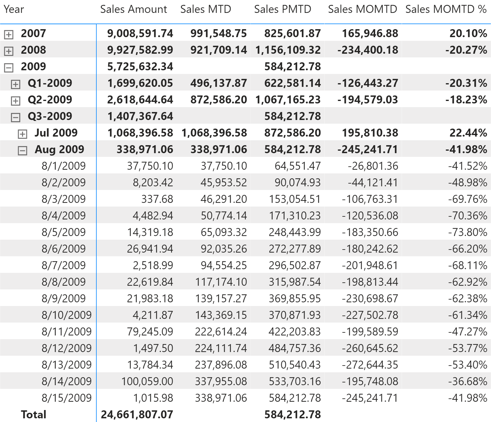
Sales PMTD uses DATEADD and filters the Date[DateWithSales] column to guarantee a fair comparison of the last period with data. Sales MOMTD and Sales MOMTD % rely on the Sales PMTD measure to guarantee the same fair comparison:
Sales PMTD :=
IF (
    [ShowValueForDates],
    CALCULATE (
        [Sales MTD],
        CALCULATETABLE (
            DATEADD ( 'Date'[Date], -1, MONTH ),
            'Date'[DateWithSales] = TRUE
        )
    )
)
Sales MOMTD :=
VAR ValueCurrentPeriod = [Sales MTD]
VAR ValuePreviousPeriod = [Sales PMTD]
VAR Result =
    IF (
        NOT ISBLANK ( ValueCurrentPeriod )
            && NOT ISBLANK ( ValuePreviousPeriod ),
        ValueCurrentPeriod - ValuePreviousPeriod
    )
RETURN
    Result
Sales MOMTD % :=
DIVIDE (
    [Sales MOMTD],
    [Sales PMTD]
)
Comparing period-to-date with previous full period
Comparing a to-date aggregation with the previous full period is useful when you consider the previous period as a benchmark. Once the current year-to-date reaches 100% of the full previous year, this means we have reached the same performance as the previous full period, hopefully in fewer days.
Year-to-date over the full previous year
The year-to-date over the full previous year compares the year-to-date against the entire previous year. Figure 12 shows that in November 2008 Sales YTD almost reaches Sales Amount for the entire year 2007. Sales YTDOPY% provides an immediate comparison of the year-to-date with the total of the previous year; it shows growth over the previous year when the percentage is positive, as is the case starting December 1, 2008.
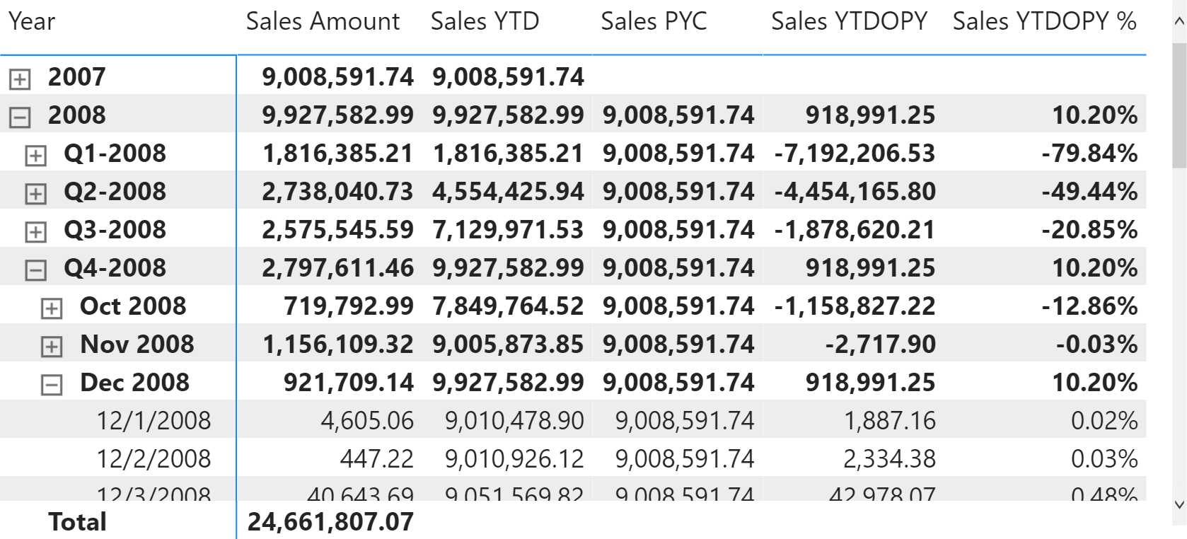
The year-to-date-over-previous-year growth is computed by the Sales YTDOPY and Sales YTDOPY % measures; these rely on the Sales YTD measure to compute the year-to-date value, and on the Sales PYC measure to get the sales amount of the entire previous year:
Sales PYC :=
IF (
    [ShowValueForDates] && HASONEVALUE ( 'Date'[Year] ),
    CALCULATE (
        [Sales Amount],
        PARALLELPERIOD ( 'Date'[Date], -1, YEAR )
    )
)
Sales YTDOPY :=
VAR ValueCurrentPeriod = [Sales YTD]
VAR ValuePreviousPeriod = [Sales PYC]
VAR Result =
    IF (
        NOT ISBLANK ( ValueCurrentPeriod )
            && NOT ISBLANK ( ValuePreviousPeriod ),
        ValueCurrentPeriod - ValuePreviousPeriod
    )
RETURN
    Result
Sales YTDOPY % :=
DIVIDE (
    [Sales YTDOPY],
    [Sales PYC]
)
The Sales PYC measure can also be written using PREVIOUSYEAR, whose behavior is similar to PARALLELPERIOD (the difference is not relevant for this example):
Sales PYC (2) :=
IF (
    [ShowValueForDates] && HASONEVALUE ( 'Date'[Year] ),
    CALCULATE (
        [Sales Amount],
        PREVIOUSYEAR ( 'Date'[Date] )
    )
)
PREVIOUSYEAR is mandatory if the comparison uses the fiscal year because PREVIOUSYEAR accepts a second argument to specify the last day of the fiscal year. Look at the following report in Figure 13, which is slicing the measures by fiscal periods.
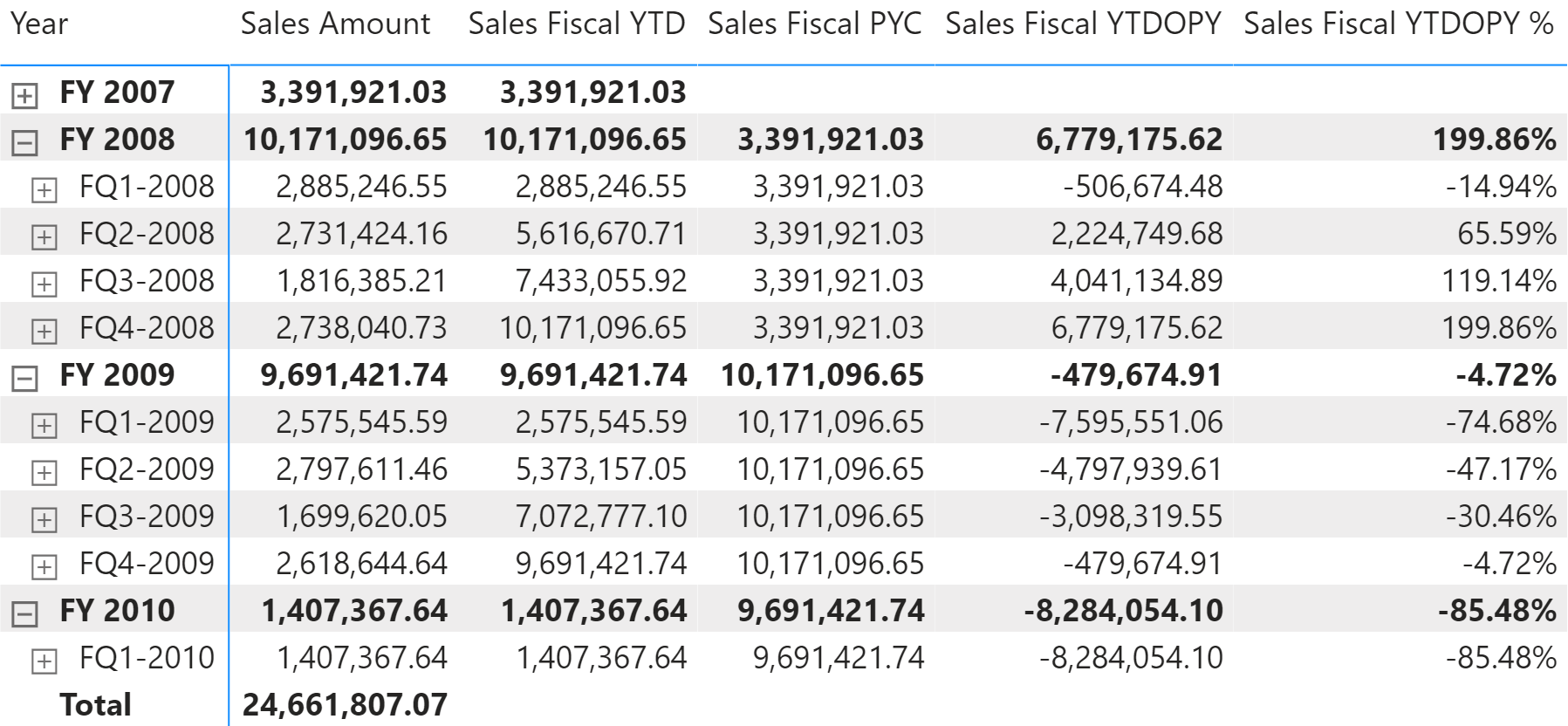
The measures used in the report are defined as follows. Please pay attention to the second argument of PREVIOUSYEAR in Sales Fiscal PYC:
Sales Fiscal PYC :=
IF (
    [ShowValueForDates],
    CALCULATE (
        [Sales Amount],
        PREVIOUSYEAR ( 'Date'[Date], "06-30" )
    )
)
Sales Fiscal YTDOPY :=
VAR ValueCurrentPeriod = [Sales Fiscal YTD]
VAR ValuePreviousPeriod = [Sales Fiscal PYC]
VAR Result =
    IF (
        NOT ISBLANK ( ValueCurrentPeriod )
            && NOT ISBLANK ( ValuePreviousPeriod ),
        ValueCurrentPeriod - ValuePreviousPeriod
    )
RETURN
    Result
Sales Fiscal YTDOPY % :=
DIVIDE (
    [Sales Fiscal YTDOPY],
    [Sales Fiscal PYC]
)
Quarter-to-date over full previous quarter
The quarter-to-date over full previous quarter compares the quarter-to-date against the entire previous quarter. Figure 14 shows that Sales QTD in May 2008 surpasses the total Sales Amount for Q1-2008. Sales QTDOPQ% provides an immediate comparison of the quarter-to-date with the total of the previous quarter; it shows growth over the previous quarter when the percentage is positive, as is the case starting in May 2008.
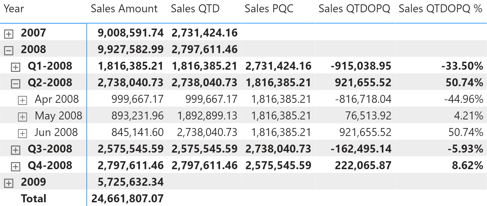
The quarter-to-date-over-previous-quarter growth is computed with the Sales QTDOPQ and Sales QTDOPQ % measures; these rely on the Sales QTD measure to compute the quarter-to-date value and on the Sales PQC measure to get the sales amount of the entire previous quarter:
Sales PQC :=
IF (
    [ShowValueForDates] && HASONEVALUE ( 'Date'[Year Quarter] ),
    CALCULATE (
        [Sales Amount],
        PARALLELPERIOD ( 'Date'[Date], -1, QUARTER )
    )
)
Sales QTDOPQ :=
VAR ValueCurrentPeriod = [Sales QTD]
VAR ValuePreviousPeriod = [Sales PQC]
VAR Result =
    IF (
        NOT ISBLANK ( ValueCurrentPeriod )
            && NOT ISBLANK ( ValuePreviousPeriod ),
        ValueCurrentPeriod - ValuePreviousPeriod
    )
RETURN
    Result
Sales QTDOPQ % :=
DIVIDE (
    [Sales QTDOPQ],
    [Sales PQC]
)
The Sales PQC measure can also be written using PREVIOUSQUARTER, as long as it is not used at the year level for more than one quarter:
Sales PQC (2) :=
IF (
    [ShowValueForDates] && HASONEVALUE ( 'Date'[Year Quarter] ),
    CALCULATE (
        [Sales Amount],
        PREVIOUSQUARTER ( 'Date'[Date] )
    )
)
Month-to-date over full previous month
The month-to-date over full previous month compares the month-to-date against the entire previous month. Figure 15 shows that Sales MTD during April 2008 surpasses the total Sales Amount for March 2008. The Sales MTDOPM% provides an immediate comparison of the month-to-date with the total of the previous month; it shows growth over the previous month when the percentage is positive as is the case starting April 19, 2008.
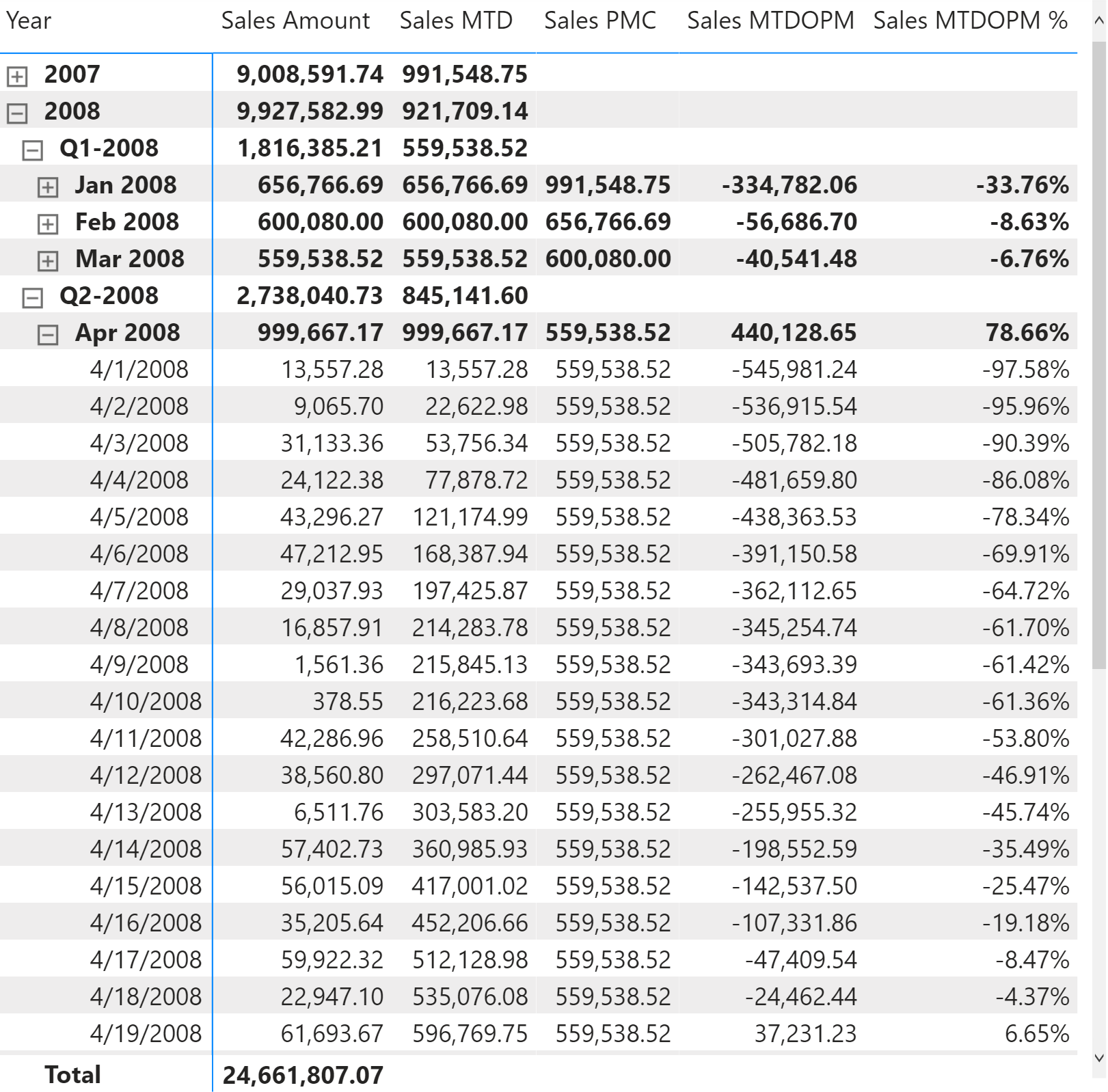
The month-to-date-over-previous-month growth is computed with the Sales MTDOPM % and Sales MTDOPM measures; these rely on the Sales MTD measure to compute the month-to-date value and on the Sales PMC measure to get the sales amount of the entire previous month:
Sales PMC :=
IF (
    [ShowValueForDates] && HASONEVALUE ( 'Date'[Year Month] ),
    CALCULATE (
        [Sales Amount],
        PARALLELPERIOD ( 'Date'[Date], -1, MONTH )
    )
)
Sales MTDOPM :=
VAR ValueCurrentPeriod = [Sales MTD]
VAR ValuePreviousPeriod = [Sales PMC]
VAR Result =
    IF (
        NOT ISBLANK ( ValueCurrentPeriod )
            && NOT ISBLANK ( ValuePreviousPeriod ),
        ValueCurrentPeriod - ValuePreviousPeriod
    )
RETURN
    Result
Sales MTDOPM % :=
DIVIDE (
    [Sales MTDOPM],
    [Sales PMC]
)
The Sales PMC measure can also be written using PREVIOUSMONTH, as long as it is not used at the quarter or year level for more than one month:
Sales PMC (2) :=
IF (
    [ShowValueForDates] && HASONEVALUE ( 'Date'[Year Month] ),
    CALCULATE (
        [Sales Amount],
        PREVIOUSMONTH ( 'Date'[Date] )
    )
)
Using moving annual total calculations
A common way to aggregate data over several months is by using the moving annual total instead of the year-to-date. The moving annual total includes the last 12 months of data. For example, the moving annual total for March 2008 includes data from April 2007 to March 2008.
Moving annual total
The Sales MAT measure computes the moving annual total, as shown in Figure 16.
The moving annual total uses DATESINPERIOD to select the previous year:
Sales MAT :=
IF (
    [ShowValueForDates],
    CALCULATE (
        [Sales Amount],
        DATESINPERIOD (
            'Date'[Date],
            MAX ( 'Date'[Date] ),
            -1,
            YEAR
        )
    )
)
DATESINPERIOD returns the set of dates starting from the date passed in the second argument and applying an offset specified in the third and fourth arguments. For example, the Sales MAT measure returns the dates included in the full year before the last date available in the filter context. The same result could have been obtained by specifying -12 and MONTH in the third and fourth arguments, respectively.
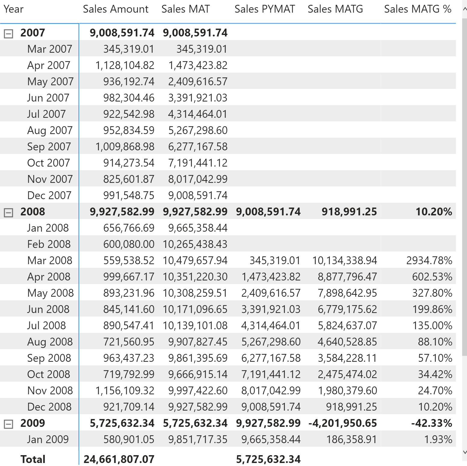
Moving annual total growth
The moving annual total growth is computed with the Sales PYMAT, Sales MATG, and Sales MATG % measures, which rely on the Sales MAT measure. The Sales MAT measure provides a correct value one year after the first sale ever (when it collects one full year of data), and it is not protected in case the current time period is shorter than a full year. For example, the amount for the full year 2009 of Sales PYMAT is 9,927,582.99, which corresponds to the Sales Amount of 2008 as shown in Figure 17. When compared with sales in 2009, this produces a comparison of less than 8 months – data being only available until August 15, 2009 – with a full year 2008. Similarly, you can see that Sales MATG % starts in 2008 with very high values and stabilizes after a year. The first values are due to the effect of having no sales in the previous year. This behavior is by design: the moving annual total is usually computed at the month or day granularity to show trends in a chart.
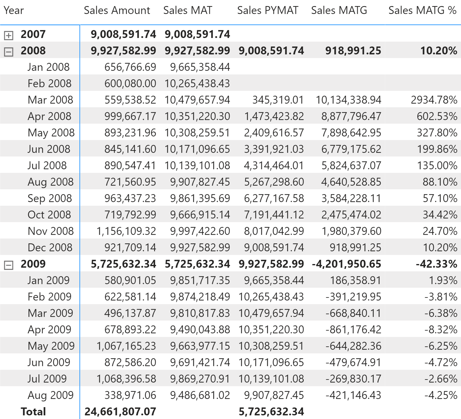
The measures are defined as follows:
Sales PYMAT :=
IF (
    [ShowValueForDates],
    CALCULATE (
        [Sales MAT],
        DATEADD ( 'Date'[Date], -1, YEAR )
    )
)
Sales MATG :=
VAR ValueCurrentPeriod = [Sales MAT]
VAR ValuePreviousPeriod = [Sales PYMAT]
VAR Result =
    IF (
        NOT ISBLANK ( ValueCurrentPeriod )
            && NOT ISBLANK ( ValuePreviousPeriod ),
        ValueCurrentPeriod - ValuePreviousPeriod
    )
RETURN
    Result
Sales MATG % :=
DIVIDE (
    [Sales MATG],
    [Sales PYMAT]
)
The Sales PYMAT measure can also be written using SAMEPERIODLASTYEAR as in the following example, which internally uses DATEADD as in the previous example:
Sales PYMAT (2) :=
IF (
    [ShowValueForDates],
    CALCULATE (
        [Sales MAT],
        SAMEPERIODLASTYEAR ( 'Date'[Date] )
    )
)
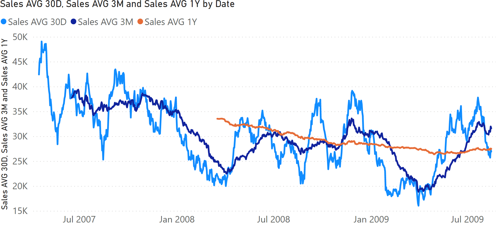
Moving averages
The moving average is typically used to display trends in line charts. Figure 18 includes the moving average of Sales Amount over 30 days (Sales AVG 30D), three months (Sales AVG 3M), and a year (Sales AVG 1Y).
Moving average 30 days
The Sales AVG 30D measure computes the moving average over 30 days by iterating a list of the last 30 dates obtained by DATESINPERIOD:
Sales AVG 30D :=
VAR Period30D =
    CALCULATETABLE (
        DATESINPERIOD (
            'Date'[Date],
            MAX ( 'Date'[Date] ),
            -30,
            DAY
        ),
        'Date'[DateWithSales] = TRUE
    )
VAR FirstDayWithData =
    CALCULATE (
        MIN ( Sales[Order Date] ),
        REMOVEFILTERS ()
    )
VAR FirstDayInPeriod =
    MINX ( Period30D, 'Date'[Date] )
VAR Result =
    IF (
        FirstDayWithData <= FirstDayInPeriod,
        AVERAGEX (
            Period30D,
            [Sales Amount]
        )
    )
RETURN
    Result
This pattern is very flexible. But for a regular additive calculation, Result can be implemented using a different and faster formula:
VAR Result =
    IF (
        FirstDayWithData <= FirstDayInPeriod,
        CALCULATE (
            DIVIDE (
                [Sales Amount],
                DISTINCTCOUNT ( Sales[Order Date] )
            ),
            Period30D
        )
    )
Moving average 3 months
The Sales AVG 3M measure computes the moving average over three months by iterating a list of the dates in the last three months obtained by DATESINPERIOD:
Sales AVG 3M :=
VAR Period3M =
    CALCULATETABLE (
        DATESINPERIOD (
            'Date'[Date],
            MAX ( 'Date'[Date] ),
            -3,
            MONTH
        ),
        'Date'[DateWithSales] = TRUE
    )
VAR FirstDayWithData =
    CALCULATE (
        MIN ( Sales[Order Date] ),
        REMOVEFILTERS ()
    )
VAR FirstDayInPeriod =
    MINX ( Period3M, 'Date'[Date] )
VAR Result =
    IF (
        FirstDayWithData <= FirstDayInPeriod,
        AVERAGEX (
            Period3M,
            [Sales Amount]
        )
    )
RETURN
    Result
For simple additive measures, the pattern based on DIVIDE which is shown for the moving average over 30 days can also be used for the average over three months.
Moving average 1 year
The Sales AVG 1Y measure computes the moving average over one year by iterating a list of the dates in the last year obtained by DATESINPERIOD:
Sales AVG 1Y :=
VAR Period1Y =
    CALCULATETABLE (
        DATESINPERIOD (
            'Date'[Date],
            MAX ( 'Date'[Date] ),
            -1,
            YEAR
        ),
        'Date'[DateWithSales] = TRUE
    )
VAR FirstDayWithData =
    CALCULATE (
        MIN ( Sales[Order Date] ),
        REMOVEFILTERS ()
    )
VAR FirstDayInPeriod =
    MINX ( Period1Y, 'Date'[Date] )
VAR Result =
    IF (
        FirstDayWithData <= FirstDayInPeriod,
        AVERAGEX (
            Period1Y,
            [Sales Amount]
        )
    )
RETURN
    Result
For simple additive measures, the same pattern based on DIVIDE, shown for the moving average over 30 days can also be used for the average over one year.
Filtering other date attributes
Once you mark the Date table as a date table, DAX automatically removes any filter from the Date table every time CALCULATE filters the date column of the Date table. This behavior is by design. Its goal is to simplify the writing of time intelligence calculations. Indeed, if DAX did not remove the filters, it would be necessary to manually add a REMOVEFILTERS over the Date table every time a DAX time intelligence function is used, resulting in a negative development experience.
The automatic removal of the filters from the Date table might introduce issues for some particular reports. For example, if a report computes the year-to-date of sales by slicing the amount by day of the week, the result obtained by only using the time intelligence function DATESYTD is wrong. Figure 19 shows that the result of Sales YTD for each day of the week is slightly smaller or equal to the row total, which is showing the value for all the days of the week.
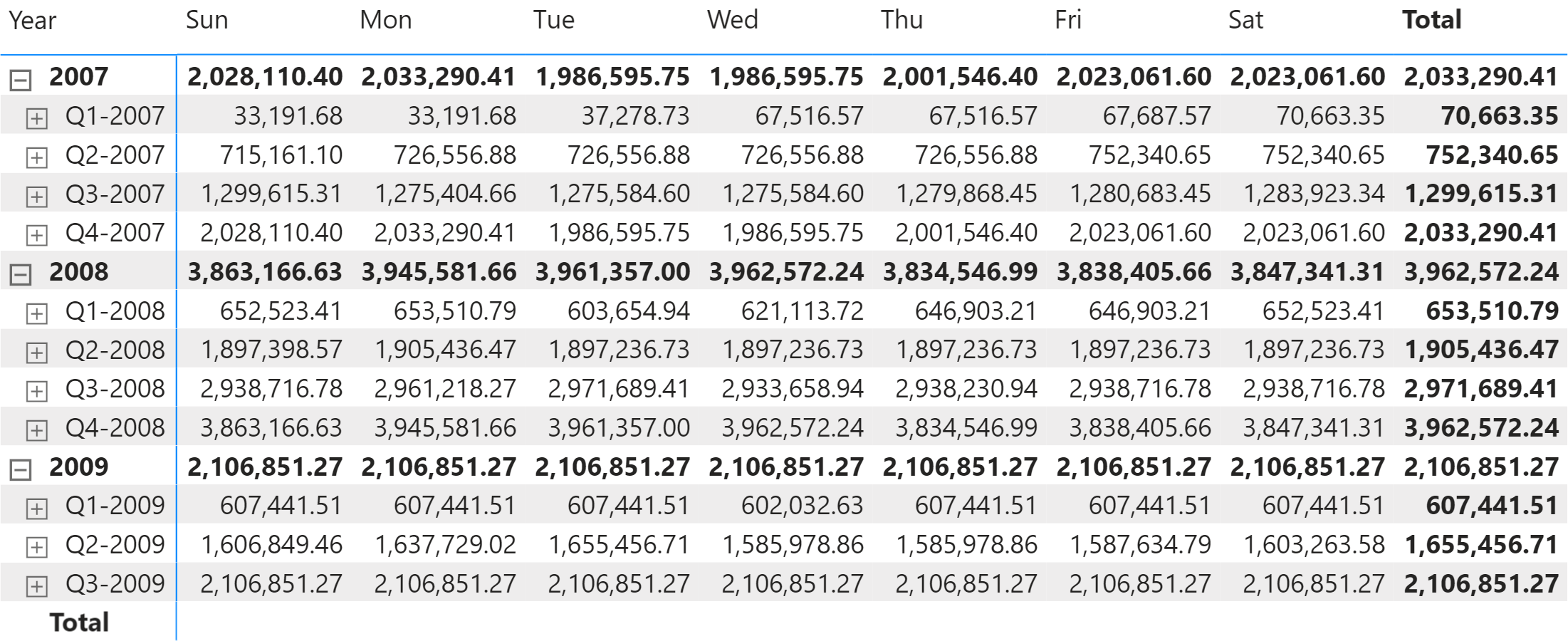
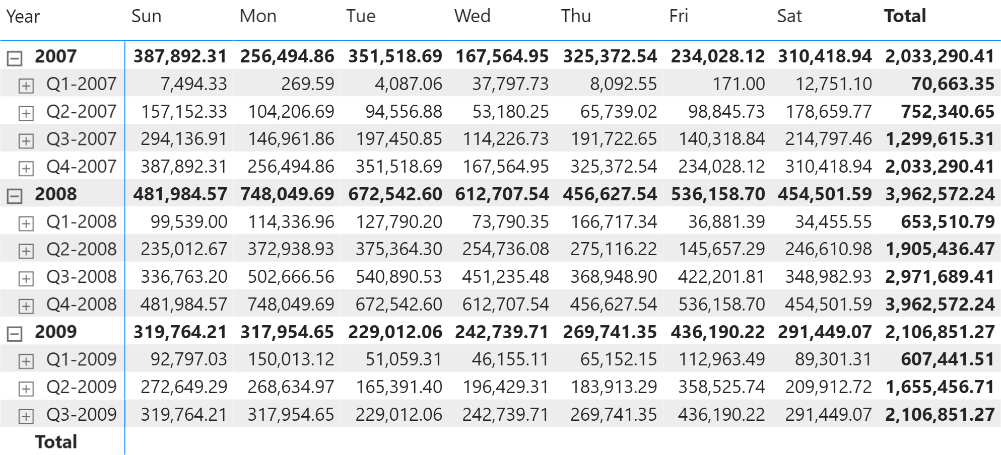
The reason for the inaccurate value is that DATESYTD applies a filter on the Date[Date] column. Because Date is marked as a date table, DAX automatically applies a REMOVEFILTERS( ‘Date’ ) modifier to the same CALCULATE where DATESYTD is used in a filter argument – thus removing the filter on the day of the week. Therefore, the number shown is the year-to-date regardless of any filter on the weekday. The day-of-week filter only affects the last day of the period specified on the rows of the report – year or quarter. The correct result, shown in Figure 20, requires a different approach.
There are two options to obtain the correct value: either reiterate the filter over the day of the week in the CALCULATE statement, or update the data model.
Restoring the filter over the day of the week requires adding VALUES ( Date[Day of Week] ) only if the columns are filtered, like in the following code:
Sales YTD (day of week) :=
IF (
    [ShowValueForDates],
    IF (
        ISFILTERED ( 'Date'[Day of Week] ),
        CALCULATE (
            [Sales Amount],
            DATESYTD ( 'Date'[Date] ),
            VALUES ( 'Date'[Day of Week] )
        ),
        CALCULATE (
            [Sales Amount],
            DATESYTD ( 'Date'[Date] )
        )
    )
)
This first solution works well, but it comes with a significant shortcoming: there are two different versions of the calculation depending on whether the Date[Day of Week] column is filtered or not. On large models, this might have a noticeable impact on performance.
There is another solution to this scenario that requires updating the data model. Instead of using the Date table to select the day of the week, we can store the day of the week in a separate table that filters Sales without being related to Date. This way, the automatic filter removal over Date does not affect the existing filter over the day of the week. For example, the Day of Week table can be created as a calculated table:
Day of Week =
SELECTCOLUMNS (
    'Date',
    "Date", 'Date'[Date],
    "Day of Week", 'Date'[Day of Week]
)
The Day of week table must have a relationship between Sales[Order Date] and ‘Day of week'[Date], meaning the model must look like the one in Figure 21.
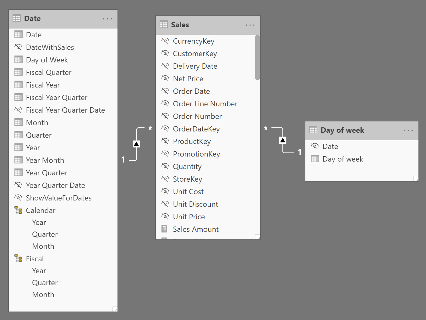
Please note that we created the new Day of Week table using all the dates in Date to create the relationship with the existing Sales[Order Date] column. It is possible to obtain the same behavior by creating a table with only seven values (Sunday through Saturday), but that choice requires an additional column in the Sales table – thus consuming more memory for the data model.
Slicing by Day of Week in the newly created table is compatible with any time intelligence calculation and respects any filter on the Day of Week table; this is because the two filters (Date and Day of the week) belong to two different tables.
The additional table could consolidate any set of attributes required by specific business rules. We built an example with the day of the week, but you can use any other set of attributes (like working days, holidays, seasons), provided that such attributes depend on Order Date.
Clear filters from the specified tables or columns.
REMOVEFILTERS ( [<TableNameOrColumnName>] [, <ColumnName> [, <ColumnName> [, … ] ] ] )
Evaluates an expression in a context modified by filters.
CALCULATE ( <Expression> [, <Filter> [, <Filter> [, … ] ] ] )
Returns a set of dates in the year up to the last date visible in the filter context.
DATESYTD ( <Dates> [, <YearEndDate>] )
Returns a table that has been filtered.
FILTER ( <Table>, <FilterExpression> )
Evaluates a table expression in a context modified by filters.
CALCULATETABLE ( <Table> [, <Filter> [, <Filter> [, … ] ] ] )
Returns the date that is the indicated number of months before or after the start date.
EDATE ( <StartDate>, <Months> )
Returns the date in datetime format of the last day of the month before or after a specified number of months.
EOMONTH ( <StartDate>, <Months> )
Convert an expression to the specified data type.
CONVERT ( <Expression>, <DataType> )
Moves the given set of dates by a specified interval.
DATEADD ( <Dates>, <NumberOfIntervals>, <Interval> )
Returns a previous day.
PREVIOUSDAY ( <Dates> )
Returns the end of month.
ENDOFMONTH ( <Dates> )
Evaluates the specified expression over the interval which begins on the first day of the year and ends with the last date in the specified date column after applying specified filters.
TOTALYTD ( <Expression>, <Dates> [, <Filter>] [, <YearEndDate>] )
Returns a set of dates in the quarter up to the last date visible in the filter context.
DATESQTD ( <Dates> )
Evaluates the specified expression over the interval which begins on the first day of the quarter and ends with the last date in the specified date column after applying specified filters.
TOTALQTD ( <Expression>, <Dates> [, <Filter>] )
Returns a set of dates in the month up to the last date visible in the filter context.
DATESMTD ( <Dates> )
Evaluates the specified expression over the interval which begins on the first of the month and ends with the last date in the specified date column after applying specified filters.
TOTALMTD ( <Expression>, <Dates> [, <Filter>] )
Returns a set of dates in the current selection from the previous year.
SAMEPERIODLASTYEAR ( <Dates> )
Returns true when the specified column is the level in a hierarchy of levels.
ISINSCOPE ( <ColumnName> )
Returns a previous year.
PREVIOUSYEAR ( <Dates> [, <YearEndDate>] )
Returns a parallel period of dates by the given set of dates and a specified interval.
PARALLELPERIOD ( <Dates>, <NumberOfIntervals>, <Interval> )
Returns a previous quarter.
PREVIOUSQUARTER ( <Dates> )
Returns a previous month.
PREVIOUSMONTH ( <Dates> )
Returns the dates from the given period.
DATESINPERIOD ( <Dates>, <StartDate>, <NumberOfIntervals>, <Interval> )
Returns a number from 1 (January) to 12 (December) representing the month.
MONTH ( <Date> )
Safe Divide function with ability to handle divide by zero case.
DIVIDE ( <Numerator>, <Denominator> [, <AlternateResult>] )
When a column name is given, returns a single-column table of unique values. When a table name is given, returns a table with the same columns and all the rows of the table (including duplicates) with the additional blank row caused by an invalid relationship if present.
VALUES ( <TableNameOrColumnName> )
This pattern is included in the book DAX Patterns, Second Edition.


Video

Do you prefer a video?
This pattern is also available in video format. Take a peek at the preview, then unlock access to the full-length video on SQLBI.com.Watch the full video — 79 min.
Downloads
Download the sample files for Power BI / Excel 2016-2019: